Once named entities have been identified in a text, we then want to extract the relations that exist between them. As indicated earlier, we will typically be looking for relations between specified types of named entity. I covered named entity recognition in a number of post. This time we will look for relations between this entities.
Load data
We will use an well established data set for relationship classification to compare our results to the state-of-the-art on this dataset. It’s the task8 dataset from SemEval 2010. You can find it here: https://github.com/davidsbatista/Annotated-Semantic-Relationships-Datasets.
with open("SemEval2010_task8_all_data/SemEval2010_task8_training/TRAIN_FILE.TXT") as f:
    train_file = f.readlines()
The training dataset consists of 8000 sentences with 10 different types of relations. Each sentence is annotated with a relation between two given nominals. The entities that are involved in this relations are identified by markers like <e1> in the text. For instance, the following sentence contains an example of the Entity-Destination relation between the nominals Flowers and chapel.
<e1>Flowers</e1> are carried into the <e2>chapel</e2>.
Using this kind of special tokens is a quite useful way to tell the network what we want it to focus on to answer our question. The main advantage is that we can use a normal text classifier architecture to tackle the relationship extraction task. This approach can be used in many different ways.
def prepare_dataset(raw):
    sentences, relations = [], []
    to_replace = [("\"", ""), ("\n", ""), ("<", " <"), (">", "> ")]
    last_was_sentence = False
    for line in raw:
        sl = line.split("\t")
        if last_was_sentence:
            relations.append(sl[0].split("(")[0].replace("\n", ""))
            last_was_sentence = False
        if sl[0].isdigit():
            sent = sl[1]
            for rp in to_replace:
                sent = sent.replace(rp[0], rp[1])
            sentences.append(sent)
            last_was_sentence = True
    print("Found {} sentences".format(len(sentences)))
    return sentences, relations
I wrote a simple function that gets us the dataset in the format we want it.
sentences, relations = prepare_dataset(train_file)
Found 8000 sentences
Now look at an example.
sentences[156]
'For those of you who are unsure what Afrikaans is, it is a language which originated from the Dutch which were the first settlers in South Africa and the unique <e1> language </e1> was evolved from other <e2> settlers </e2> from Malaya, Indonesia, Madagascar and West Africa.'
relations[156]
'Entity-Origin'
n_relations = len(set(relations))
print("Found {} relations\n".format(n_relations))
print("Relations:\n{}".format(list(set(relations))))
Found 10 relations

Relations:
['Instrument-Agency', 'Message-Topic', 'Content-Container', 'Entity-Origin', 'Product-Producer', 'Entity-Destination', 'Cause-Effect', 'Component-Whole', 'Other', 'Member-Collection']
Implement the attention mechanism
In the recent years the so called attention mechanism has had quite a lot of success. This attention layer basically learns a weighting of the input sequence and averages the sequence accordingly to extract the relevant information. I walk you through the math and show you how to implement it.
Let $h$ be a matrix consisting of output vectors $[h_1, h_2, \dots, h_T]$ that the biLSTM layer produced, where $T$ is the sentence length. The representation $r$ of the sentence is formed by a weighted sum of these output vectors: $$\alpha = \text{softmax}(w^Th)$$ $$r = h\alpha^T,$$ where $h\in\mathbb{R}^{d^w\times T}$, $d^w$ is the dimension of the word vectors, $w$ is a trained parameter vector and $w^T$ is the transpose. The dimension of $w$, $\alpha$, $r$ is $d^w$, $T$ and $d^w$ respectively. We obtain the final sentence-pair representation used for classification from: $$h^∗ = \text{tanh}(r).$$
Let me show you the important parts of the implementation. You can find the full code on my github here. The magic happens in the call function of the keras class.
def call(self, h, mask=None):
    h_shape = K.shape(h)
    d_w, T = h_shape[0], h_shape[1]

    logits = K.dot(h, self.w)  # w^T h
    logits = K.reshape(logits, (d_w, T))
    alpha = K.exp(logits - K.max(logits, axis=-1, keepdims=True))  # exp
    alpha = alpha / K.sum(alpha, axis=1, keepdims=True)  # softmax
    r = K.sum(h * K.expand_dims(alpha), axis=1)  # r = h*alpha^T
    h_star = K.tanh(r)  # h^* = tanh(r)
    return h_star
Setup a sequence model
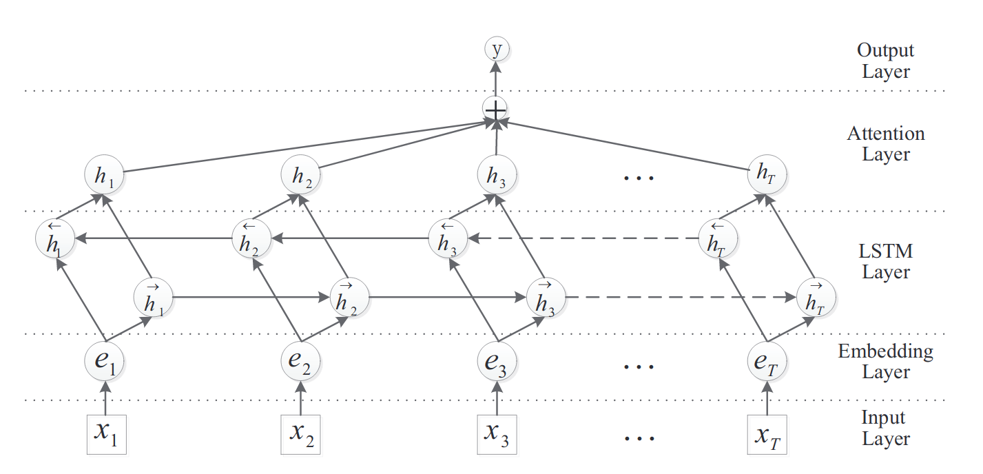
We use my custom keras text classifier here. You can find the code on my github. Key here is, that we use a bidirectional LSTM model with an Attention layer on top. This allows the model to explicitly focus on certain parts of the input and we can visualize the attention of the model later. The architecture reads as follows:
- Input layer: input sentence to this model;
- Embedding layer: map each word into a low-dimension vector;
- LSTM layer: utilize biLSTM to get high level features from step 2.;
- Attention layer: produce a weight vector and merge word-level features from each time step into a sentence-level feature vector, by multiplying the weight vector;
- Output layer: the sentence-level feature vector is finally used for relation classification.
You can find the code for this model here.
from models import KerasTextClassifier
import numpy as np
from sklearn.model_selection import train_test_split
Using TensorFlow backend.
kclf = KerasTextClassifier(input_length=50, n_classes=n_relations, max_words=15000)
tr_sent, te_sent, tr_rel, te_rel = train_test_split(sentences, relations, test_size=0.1)
kclf.fit(X=tr_sent, y=tr_rel, X_val=te_sent, y_val=te_rel,
         batch_size=10, lr=0.001, epochs=20)
Fit text model with 10 classes
Train on 7200 samples, validate on 800 samples
Epoch 1/20
7200/7200 [==============================] - 112s 16ms/step - loss: 2.1497 - acc: 0.2244 - val_loss: 1.9443 - val_acc: 0.2675
Epoch 2/20
7200/7200 [==============================] - 109s 15ms/step - loss: 1.8508 - acc: 0.3379 - val_loss: 1.7216 - val_acc: 0.3813
Epoch 3/20
7200/7200 [==============================] - 109s 15ms/step - loss: 1.6728 - acc: 0.4021 - val_loss: 1.5716 - val_acc: 0.4175
Epoch 4/20
7200/7200 [==============================] - 109s 15ms/step - loss: 1.5261 - acc: 0.4442 - val_loss: 1.4190 - val_acc: 0.4788
Epoch 5/20
7200/7200 [==============================] - 109s 15ms/step - loss: 1.4255 - acc: 0.4829 - val_loss: 1.3338 - val_acc: 0.5088
Epoch 6/20
7200/7200 [==============================] - 109s 15ms/step - loss: 1.3172 - acc: 0.5231 - val_loss: 1.2522 - val_acc: 0.5463
Epoch 7/20
7200/7200 [==============================] - 109s 15ms/step - loss: 1.2399 - acc: 0.5568 - val_loss: 1.2022 - val_acc: 0.5588
Epoch 8/20
7200/7200 [==============================] - 109s 15ms/step - loss: 1.1453 - acc: 0.5951 - val_loss: 1.1971 - val_acc: 0.5863
Epoch 9/20
7200/7200 [==============================] - 109s 15ms/step - loss: 1.0774 - acc: 0.6168 - val_loss: 1.1309 - val_acc: 0.5925
Epoch 10/20
7200/7200 [==============================] - 109s 15ms/step - loss: 1.0043 - acc: 0.6525 - val_loss: 1.0923 - val_acc: 0.6188
Epoch 11/20
7200/7200 [==============================] - 109s 15ms/step - loss: 0.9163 - acc: 0.6857 - val_loss: 1.0720 - val_acc: 0.6363
Epoch 12/20
7200/7200 [==============================] - 109s 15ms/step - loss: 0.8765 - acc: 0.6976 - val_loss: 1.0892 - val_acc: 0.6325
Epoch 13/20
7200/7200 [==============================] - 109s 15ms/step - loss: 0.8226 - acc: 0.7208 - val_loss: 1.0617 - val_acc: 0.6625
Epoch 14/20
7200/7200 [==============================] - 109s 15ms/step - loss: 0.7670 - acc: 0.7410 - val_loss: 1.0577 - val_acc: 0.6500
Epoch 15/20
7200/7200 [==============================] - 109s 15ms/step - loss: 0.7164 - acc: 0.7631 - val_loss: 1.1130 - val_acc: 0.6538
Epoch 16/20
7200/7200 [==============================] - 109s 15ms/step - loss: 0.6763 - acc: 0.7778 - val_loss: 1.1417 - val_acc: 0.6463
Epoch 17/20
7200/7200 [==============================] - 109s 15ms/step - loss: 0.6347 - acc: 0.7915 - val_loss: 1.1191 - val_acc: 0.6613
Epoch 18/20
7200/7200 [==============================] - 109s 15ms/step - loss: 0.6074 - acc: 0.8046 - val_loss: 1.1286 - val_acc: 0.6650
Epoch 19/20
7200/7200 [==============================] - 109s 15ms/step - loss: 0.5638 - acc: 0.8150 - val_loss: 1.2018 - val_acc: 0.6613
Epoch 20/20
7200/7200 [==============================] - 109s 15ms/step - loss: 0.5360 - acc: 0.8243 - val_loss: 1.1860 - val_acc: 0.6663
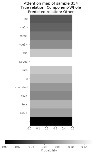
Investigate Attention
The weights learned by the attention layer can be investigated to understand what the model is focusing on. Let’s have a look.
import matplotlib.pyplot as plt
plt.style.use("ggplot")
%matplotlib inline
y_pred = kclf.predict(te_sent)
y_attn = kclf._get_attention_map(te_sent)
i = 354
activation_map = np.expand_dims(y_attn[i][:len(te_sent[i].split())], axis=1)

f = plt.figure(figsize=(8, 8))
ax = f.add_subplot(1, 1, 1)

img = ax.imshow(activation_map, interpolation='none', cmap='gray')

plt.xlim([0,0.5])
ax.set_aspect(0.1)
ax.set_yticks(range(len(te_sent[i].split())))
ax.set_yticklabels(te_sent[i].split());
ax.grid()
plt.title("Attention map of sample {}\nTrue relation: {}\nPredicted relation: {}"
          .format(i, te_rel[i], kclf.encoder.classes_[y_pred[i]]));

# add colorbar
cbaxes = f.add_axes([0.2, 0, 0.6, 0.03]);
cbar = f.colorbar(img, cax=cbaxes, orientation='horizontal');
cbar.ax.set_xlabel('Probability', labelpad=2);
Evaluate the model
We want to compare your model to the state-of-the-art. This paper from 2016 reports a macro F1-Score of 0.844. If you find a more recent source please tell me. So we will load the official test data and try to beat them.
from sklearn.metrics import f1_score, classification_report, accuracy_score
y_test_pred = kclf.predict(te_sent)
label_idx_to_use = [i for i, c in enumerate(list(kclf.encoder.classes_)) if  c !="Other"]
label_to_use = list(kclf.encoder.classes_)
label_to_use.remove("Other")
print("F1-Score: {:.1%}"
      .format(f1_score(kclf.encoder.transform(te_rel), y_test_pred,
                       average="macro", labels=label_idx_to_use)))
F1-Score: 71.7%
print(classification_report(kclf.encoder.transform(te_rel), y_test_pred,
                            target_names=label_to_use,
                            labels=label_idx_to_use))
                    precision    recall  f1-score   support

      Cause-Effect       0.79      0.81      0.80        94
   Component-Whole       0.68      0.60      0.64       102
 Content-Container       0.75      0.76      0.76        51
Entity-Destination       0.80      0.82      0.81        65
     Entity-Origin       0.76      0.88      0.82        66
 Instrument-Agency       0.68      0.51      0.58        55
 Member-Collection       0.80      0.93      0.86        84
     Message-Topic       0.70      0.53      0.61        58
  Product-Producer       0.50      0.70      0.58        77

       avg / total       0.72      0.73      0.72       652
It looks we are quite a margin away from the specialized state-of-the-art models. Try to improve the model with pre-trained wordvectors or a better regularization strategy. I hope you like what you learned in this post and stay tuned for more.