In this post, I will show you how to use the isolation forest algorithm to detect attacks to computer networks in python.
The term isolation means separating an instance from the rest of the instances. Since anomalies are ‘few and different’ and therefore they are more susceptible to isolation. In a data-induced random tree, partitioning of instances are repeated recursively until all instances are isolated. This random partitioning produces noticeable shorter paths for anomalies since the fewer instances of anomalies result in a smaller number of partitions – shorter paths in a tree structure, and instances with distinguishable attribute-values are more likely to be separated in early partitioning. Hence, when a forest of random trees collectively produce shorter path lengths for some particular points, then they are highly likely to be anomalies. We denote anomalies by $x_o$ and normal datapoints by $x_i$.
The dataset
We use the Http dataset from the KDDCUP in 1999. The dataset contains 623091 http connection records from seven weeks of network traffic. A connection is a sequence of TCP packets starting and ending at some well defined times, between which data flows to and from a source IP address to a target IP address under some well defined protocol. The dataset is already preprocessed and contains 41 features of the individual TCP connections, content features and traffic features. Each connection is labeled as either normal, or as an attack, with exactly one specific attack type.
We want to build a unsupervised model to detect the attacks.
cols = ["duration", "protocol_type", "service", "flag", "src_bytes", "dst_bytes", "land", "wrong_fragment", "urgent",
        "hot", "num_failed_logins", "logged_in", "num_compromised", "root_shell", "su_attempted", "num_root",
        "num_file_creations", "num_shells", "num_access_files", "num_outbound_cmds", "is_host_login",
        "is_guest_login", "count", "srv_count", "serror_rate", "srv_serror_rate", "rerror_rate", "srv_rerror_rate",
        "same_srv_rate", "diff_srv_rate", "srv_diff_host_rate", "dst_host_count", "dst_host_srv_count",
        "dst_host_same_srv_rate", "dst_host_diff_srv_rate", "dst_host_same_src_port_rate", "dst_host_srv_diff_host_rate",
        "dst_host_serror_rate", "dst_host_srv_serror_rate", "dst_host_rerror_rate", "dst_host_srv_rerror_rate"]
import pandas as pd
import numpy as np
import matplotlib.pyplot as plt
plt.style.use("ggplot")
%matplotlib inline

df = pd.read_csv("data/kddcup.data.corrected", sep=",", names=cols + ["label"], index_col=None)
df = df[df["service"] == "http"]
df = df.drop("service", axis=1)
cols.remove("service")
df.shape
(623091, 41)
df.head()
| duration | protocol_type | flag | src_bytes | dst_bytes | land | wrong_fragment | urgent | hot | num_failed_logins | ... | dst_host_srv_count | dst_host_same_srv_rate | dst_host_diff_srv_rate | dst_host_same_src_port_rate | dst_host_srv_diff_host_rate | dst_host_serror_rate | dst_host_srv_serror_rate | dst_host_rerror_rate | dst_host_srv_rerror_rate | label | |
|---|---|---|---|---|---|---|---|---|---|---|---|---|---|---|---|---|---|---|---|---|---|
| 0 | 0 | tcp | SF | 215 | 45076 | 0 | 0 | 0 | 0 | 0 | ... | 0 | 0.0 | 0.0 | 0.00 | 0.0 | 0.0 | 0.0 | 0.0 | 0.0 | normal. |
| 1 | 0 | tcp | SF | 162 | 4528 | 0 | 0 | 0 | 0 | 0 | ... | 1 | 1.0 | 0.0 | 1.00 | 0.0 | 0.0 | 0.0 | 0.0 | 0.0 | normal. |
| 2 | 0 | tcp | SF | 236 | 1228 | 0 | 0 | 0 | 0 | 0 | ... | 2 | 1.0 | 0.0 | 0.50 | 0.0 | 0.0 | 0.0 | 0.0 | 0.0 | normal. |
| 3 | 0 | tcp | SF | 233 | 2032 | 0 | 0 | 0 | 0 | 0 | ... | 3 | 1.0 | 0.0 | 0.33 | 0.0 | 0.0 | 0.0 | 0.0 | 0.0 | normal. |
| 4 | 0 | tcp | SF | 239 | 486 | 0 | 0 | 0 | 0 | 0 | ... | 4 | 1.0 | 0.0 | 0.25 | 0.0 | 0.0 | 0.0 | 0.0 | 0.0 | normal. |
5 rows × 41 columns
Now we need to encode the categorical columns.
from sklearn.preprocessing import LabelEncoder

encs = dict()
data = df.copy()  #.sample(frac=1)
for c in data.columns:
    if data[c].dtype == "object":
        encs[c] = LabelEncoder()
        data[c] = encs[c].fit_transform(data[c])
Implementing the isolation forest
While the implementation of the isolation forest algorithm is straigth forward, we use the implementation of the scikit-learn python package. Let’s see how it works. The isolation forest algorithm has several hyperparmaters which we will discuss.
- n_estimators: The number of trees to use. The paper suggests an number of 100 trees, because the path lengths usually converges well before that.
- max_samples: The number of samples to draw while build a single tree. This parameter is called sub-sampeling in the paper and they suggest max_samples=256, since it generally provides enough details to perform anomaly detection across a wide range of data.
- contamination: The amount of contamination of the data set, i.e. the proportion of outliers in the data set. Used when fitting to define the threshold on the decision function. I will show you how to pick this treshold later.
from sklearn.ensemble import IsolationForest
We split the data in train, validation and test data.
X_train, y_train = data[cols][:300000], data["label"][:300000].values
X_valid, y_valid = data[cols][300000:500000], data["label"][300000:500000].values
X_test, y_test = data[cols][500000:], data["label"][500000:].values
Now we set up the isolation forest model and fit it. We set the contamination parameter to 20% (because it cannot be 0, this will not affect the fitting of the trees) for now and set a threshold on the average path length later.
iForest = IsolationForest(n_estimators=100, max_samples=256, contamination=0.2, random_state=2018)
iForest.fit(X_train)
IsolationForest(bootstrap=False, contamination=0.2, max_features=1.0,
        max_samples=256, n_estimators=100, n_jobs=1, random_state=2018,
        verbose=0)
Finding anomalies
The .decision_function of the isolation forest provides a score that is derived from the the average path lengths of the samples in the model. We can use this to decide which samples are anomalies.
scores = iForest.decision_function(X_valid)
plt.figure(figsize=(12, 8))
plt.hist(scores, bins=50);
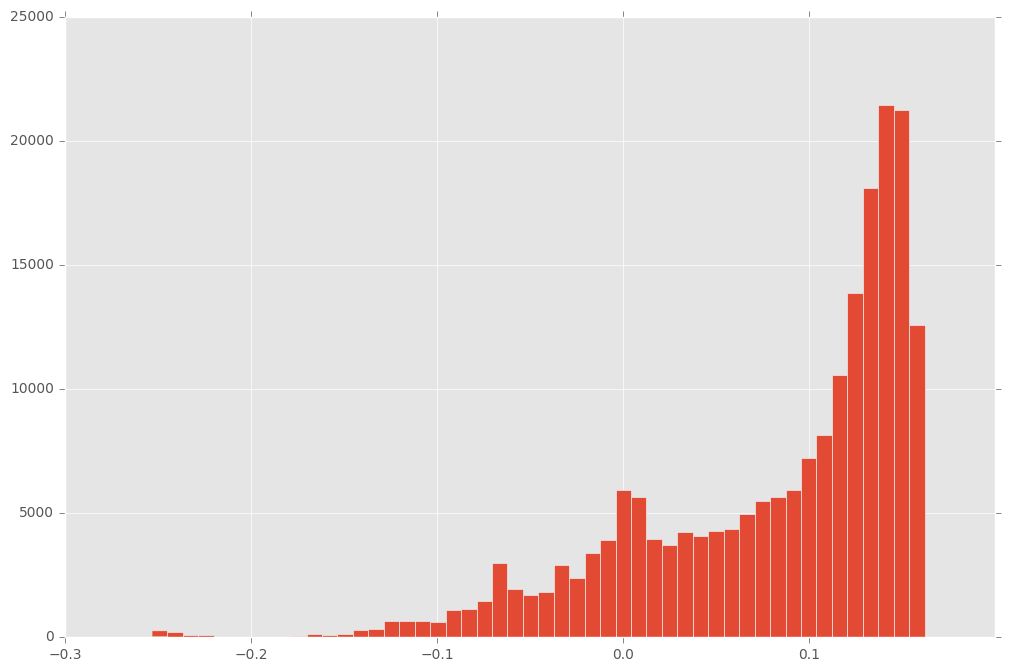
So we see, that there is a clear cluster under -0.2. We consider average path lengths shorter than -0.2 as anomalies. How would this perform on the validation data?
from sklearn.metrics import roc_auc_score

print("AUC: {:.1%}".format(roc_auc_score((-0.2 < scores), y_valid == list(encs["label"].classes_).index("normal."))))
AUC: 99.0%
This is pretty good! Now we check the numbers on some of the test data.
scores_test = iForest.decision_function(X_test)
print("AUC: {:.1%}".format(roc_auc_score((-0.2 < scores_test),
                                         y_test == list(encs["label"].classes_).index("normal."))))
AUC: 99.3%
Also really good! So now you saw how to perform anomaly detection with isolation forests in python.
Further reading