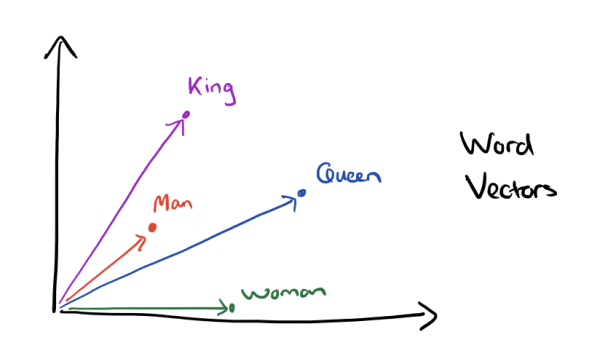
Word vectors
Today, I tell you what word vectors are, how you create them in python and finally how you can use them with neural networks in keras. For a long time, NLP methods use a vectorspace model to represent words. Commonly one-hot encoded vectors are used. This traditional, so called Bag of Words approach is pretty successful for a lot of tasks.
Recently, new methods for representing words in a vectorspace have been proposed and yielded big improvements in a lot of different NLP tasks. We will discuss some of these methods and see how to create this vectors in python.
Continous Bag of Words
The basic idea grounds in the distributional hypothises, which states that the meaning of a word can be inferred from it’s surrounding words. So the idea of the continuous bag of words (CBOW) is to use the context of a word to predict the probability that this word appears.
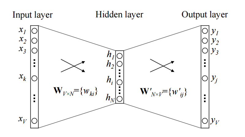
The image shows a simple CBOW model with only one word in the context window. So the input is a one-hot encoded context word and a hidden size of $N$ and a vocabulary size of $V$. After training this little network the columns of $W^\prime$ contains a $N$-dimensional vector representation for every word in the vocabulary. This is what we use as word vector.
For more details I recommend to read the following:
- Xin Rong: “word2vec Parameter Learning Explained”
- Yoav Goldberg and Omer Levy: “word2vec Explained: Deriving Mikolov et al.’s Negative-Sampling Word-Embedding Method”
Or directly the main papers:
- Efficient Estimation of Word Representations in Vector Space – Mikolov et al. 2013
- Distributed Representations of Words and Phrases and their Compositionality – Mikolov et al. 2013
A great blog post for this topic you can find here.
Load dataset
We use the dataset from the “Toxic Comment Classification Challenge”, a recent kaggle competition, where you’re challenged to build a multi-headed model that’s capable of detecting different types of of toxicity like threats, obscenity, insults, and identity-based hate. We first preprocess the comments, and train word vectors. Then we initialize a keras embedding layer with the pretrained word vectors and compare the performance with an randomly initialized embedding. On top of the embeddings an LSTM with dropout is used.
import pandas as pd
import numpy as np

import matplotlib.pyplot as plt
plt.style.use("ggplot")
path = 'data/'

TRAIN_DATA_FILE = path + 'train.csv'
TEST_DATA_FILE = path + 'test.csv'
train_df = pd.read_csv(TRAIN_DATA_FILE)
test_df = pd.read_csv(TEST_DATA_FILE)
train_df.head(10)
| id | comment_text | toxic | severe_toxic | obscene | threat | insult | identity_hate | |
|---|---|---|---|---|---|---|---|---|
| 0 | 0000997932d777bf | Explanation\nWhy the edits made under my usern... | 0 | 0 | 0 | 0 | 0 | 0 |
| 1 | 000103f0d9cfb60f | D'aww! He matches this background colour I'm s... | 0 | 0 | 0 | 0 | 0 | 0 |
| 2 | 000113f07ec002fd | Hey man, I'm really not trying to edit war. It... | 0 | 0 | 0 | 0 | 0 | 0 |
| 3 | 0001b41b1c6bb37e | "\nMore\nI can't make any real suggestions on ... | 0 | 0 | 0 | 0 | 0 | 0 |
| 4 | 0001d958c54c6e35 | You, sir, are my hero. Any chance you remember... | 0 | 0 | 0 | 0 | 0 | 0 |
| 5 | 00025465d4725e87 | "\n\nCongratulations from me as well, use the ... | 0 | 0 | 0 | 0 | 0 | 0 |
| 6 | 0002bcb3da6cb337 | COCKSUCKER BEFORE YOU PISS AROUND ON MY WORK | 1 | 1 | 1 | 0 | 1 | 0 |
| 7 | 00031b1e95af7921 | Your vandalism to the Matt Shirvington article... | 0 | 0 | 0 | 0 | 0 | 0 |
| 8 | 00037261f536c51d | Sorry if the word 'nonsense' was offensive to ... | 0 | 0 | 0 | 0 | 0 | 0 |
| 9 | 00040093b2687caa | alignment on this subject and which are contra... | 0 | 0 | 0 | 0 | 0 | 0 |
Preprocess the text
Now we preprocess the comments. For this we replace URLs by “URL” and IP addresses by “IPADDRESS”. Then we tokenize the text and lowercase it.
########################################
## process texts in datasets
########################################
print('Processing text dataset')
from nltk.tokenize import WordPunctTokenizer
from collections import Counter
from string import punctuation, ascii_lowercase
import regex as re
from tqdm import tqdm

# replace urls
re_url = re.compile(r"((http|https)\:\/\/)?[a-zA-Z0-9\.\/\?\:@\-_=#]+\
                    .([a-zA-Z]){2,6}([a-zA-Z0-9\.\&\/\?\:@\-_=#])*",
                    re.MULTILINE|re.UNICODE)
# replace ips
re_ip = re.compile("\d{1,3}\.\d{1,3}\.\d{1,3}\.\d{1,3}")

# setup tokenizer
tokenizer = WordPunctTokenizer()

vocab = Counter()

def text_to_wordlist(text, lower=False):
    # replace URLs
    text = re_url.sub("URL", text)

    # replace IPs
    text = re_ip.sub("IPADDRESS", text)

    # Tokenize
    text = tokenizer.tokenize(text)

    # optional: lower case
    if lower:
        text = [t.lower() for t in text]

    # Return a list of words
    vocab.update(text)
    return text

def process_comments(list_sentences, lower=False):
    comments = []
    for text in tqdm(list_sentences):
        txt = text_to_wordlist(text, lower=lower)
        comments.append(txt)
    return comments


list_sentences_train = list(train_df["comment_text"].fillna("NAN_WORD").values)
list_sentences_test = list(test_df["comment_text"].fillna("NAN_WORD").values)

comments = process_comments(list_sentences_train + list_sentences_test, lower=True)
Processing text dataset


100%|██████████| 312735/312735 [00:17<00:00, 18030.28it/s]
print("The vocabulary contains {} unique tokens".format(len(vocab)))
The vocabulary contains 365516 unique tokens
Model the word vectors with Gensim
Now we are ready to train the word vectors. We use the gensim library in python which supports a bunch of classes for NLP applications. As discussed, we use a CBOW model with negative sampling and 100 dimensional word vectors.
from gensim.models import Word2Vec
model = Word2Vec(comments, size=100, window=5, min_count=5, workers=16, sg=0, negative=5)
word_vectors = model.wv
print("Number of word vectors: {}".format(len(word_vectors.vocab)))
Number of word vectors: 70056
Let’s see if we have trained semantically reasonable word vectors.
model.wv.most_similar_cosmul(positive=['woman', 'king'], negative=['man'])
[('prince', 0.9849334359169006),
 ('queen', 0.9684107899665833),
 ('princess', 0.9518582820892334),
 ('bishop', 0.9380313158035278),
 ('duke', 0.9368391633033752),
 ('duchess', 0.9353090524673462),
 ('victoria', 0.920809805393219),
 ('mary', 0.9180552363395691),
 ('mayor', 0.912704348564148),
 ('prussia', 0.9100297093391418)]
That looks really good! Now we can go on to the text classification model.
Initialize the embeddings in keras
First we have to pad or cut the tokenized comments to a certain length.
MAX_NB_WORDS = len(word_vectors.vocab)
MAX_SEQUENCE_LENGTH = 200
from keras.preprocessing.sequence import pad_sequences

word_index = {t[0]: i+1 for i,t in enumerate(vocab.most_common(MAX_NB_WORDS))}
sequences = [[word_index.get(t, 0) for t in comment]
             for comment in comments[:len(list_sentences_train)]]
test_sequences = [[word_index.get(t, 0)  for t in comment]
                  for comment in comments[len(list_sentences_train):]]

# pad
data = pad_sequences(sequences, maxlen=MAX_SEQUENCE_LENGTH,
                     padding="pre", truncating="post")
list_classes = ["toxic", "severe_toxic", "obscene", "threat", "insult", "identity_hate"]
y = train_df[list_classes].values
print('Shape of data tensor:', data.shape)
print('Shape of label tensor:', y.shape)

test_data = pad_sequences(test_sequences, maxlen=MAX_SEQUENCE_LENGTH, padding="pre",
                          truncating="post")
print('Shape of test_data tensor:', test_data.shape)
Using TensorFlow backend.


Shape of data tensor: (159571, 200)
Shape of label tensor: (159571, 6)
Shape of test_data tensor: (153164, 200)
Now we finally create the embedding matrix. This is what we will feed to the keras embedding layer. Note, that you can use the same code to easily initialize the embeddings with Glove or other pretrained word vectors.
WV_DIM = 100
nb_words = min(MAX_NB_WORDS, len(word_vectors.vocab))
# we initialize the matrix with random numbers
wv_matrix = (np.random.rand(nb_words, WV_DIM) - 0.5) / 5.0
for word, i in word_index.items():
    if i >= MAX_NB_WORDS:
        continue
    try:
        embedding_vector = word_vectors[word]
        # words not found in embedding index will be all-zeros.
        wv_matrix[i] = embedding_vector
    except:
        pass
Setup the comment classifier
from keras.layers import Dense, Input, CuDNNLSTM, Embedding, Dropout,SpatialDropout1D, Bidirectional
from keras.models import Model
from keras.optimizers import Adam
from keras.layers.normalization import BatchNormalization
We use a bidirectional LSTM with dropout and batch normalization. Note that we use the CUDA implementation of keras, which runs much faster on GPU than the normal LSTM layer.
wv_layer = Embedding(nb_words,
                     WV_DIM,
                     mask_zero=False,
                     weights=[wv_matrix],
                     input_length=MAX_SEQUENCE_LENGTH,
                     trainable=False)

# Inputs
comment_input = Input(shape=(MAX_SEQUENCE_LENGTH,), dtype='int32')
embedded_sequences = wv_layer(comment_input)

# biGRU
embedded_sequences = SpatialDropout1D(0.2)(embedded_sequences)
x = Bidirectional(CuDNNLSTM(64, return_sequences=False))(embedded_sequences)

# Output
x = Dropout(0.2)(x)
x = BatchNormalization()(x)
preds = Dense(6, activation='sigmoid')(x)

# build the model
model = Model(inputs=[comment_input], outputs=preds)
model.compile(loss='binary_crossentropy',
              optimizer=Adam(lr=0.001, clipnorm=.25, beta_1=0.7, beta_2=0.99),
              metrics=[])
hist = model.fit([data], y, validation_split=0.1,
                 epochs=10, batch_size=256, shuffle=True)
Train on 143613 samples, validate on 15958 samples
Epoch 1/10
143613/143613 [==============================] - 15s 103us/step - loss: 0.1681 - val_loss: 0.0551
Epoch 2/10
143613/143613 [==============================] - 14s 97us/step - loss: 0.0574 - val_loss: 0.0502
Epoch 3/10
143613/143613 [==============================] - 14s 97us/step - loss: 0.0522 - val_loss: 0.0486
Epoch 4/10
143613/143613 [==============================] - 14s 96us/step - loss: 0.0501 - val_loss: 0.0466
Epoch 5/10
143613/143613 [==============================] - 14s 97us/step - loss: 0.0472 - val_loss: 0.0464
Epoch 6/10
143613/143613 [==============================] - 14s 97us/step - loss: 0.0460 - val_loss: 0.0448
Epoch 7/10
143613/143613 [==============================] - 14s 97us/step - loss: 0.0448 - val_loss: 0.0448
Epoch 8/10
143613/143613 [==============================] - 14s 97us/step - loss: 0.0438 - val_loss: 0.0453
Epoch 9/10
143613/143613 [==============================] - 14s 98us/step - loss: 0.0431 - val_loss: 0.0446
Epoch 10/10
143613/143613 [==============================] - 14s 97us/step - loss: 0.0425 - val_loss: 0.0454
Let’s look at the training loss compared to the validation loss.
history = pd.DataFrame(hist.history)
plt.figure(figsize=(12,12));
plt.plot(history["loss"]);
plt.plot(history["val_loss"]);
plt.title("Loss with pretrained word vectors");
plt.show();
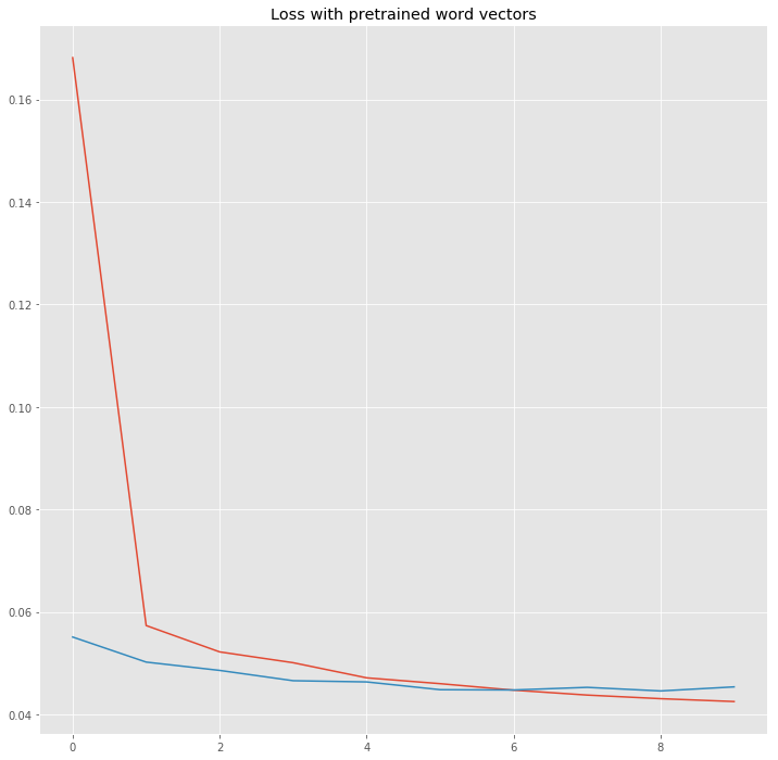
It looks like the loss is decreasing nicely, but there is still room for improvement. You can try to play with the embeddings, the dropout and the architecture of the network. Now we want to compare the pretrained word vectors with randomly initialized embeddings.
wv_layer = Embedding(nb_words,
                     WV_DIM,
                     mask_zero=False,
                     # weights=[wv_matrix],
                     input_length=MAX_SEQUENCE_LENGTH,
                     trainable=False)

# Inputs
comment_input = Input(shape=(MAX_SEQUENCE_LENGTH,), dtype='int32')
embedded_sequences = wv_layer(comment_input)

# biGRU
embedded_sequences = SpatialDropout1D(0.2)(embedded_sequences)
x = Bidirectional(CuDNNLSTM(64, return_sequences=False))(embedded_sequences)

# Output
x = Dropout(0.2)(x)
x = BatchNormalization()(x)
preds = Dense(6, activation='sigmoid')(x)

# build the model
model = Model(inputs=[comment_input], outputs=preds)
model.compile(loss='binary_crossentropy',
              optimizer=Adam(lr=0.001, clipnorm=.25, beta_1=0.7, beta_2=0.99),
              metrics=[])
hist = model.fit([data], y, validation_split=0.1,
                 epochs=10, batch_size=256, shuffle=True)
Train on 143613 samples, validate on 15958 samples
Epoch 1/10
143613/143613 [==============================] - 14s 99us/step - loss: 0.1800 - val_loss: 0.1085
Epoch 2/10
143613/143613 [==============================] - 14s 97us/step - loss: 0.1117 - val_loss: 0.1063
Epoch 3/10
143613/143613 [==============================] - 14s 98us/step - loss: 0.1063 - val_loss: 0.0990
Epoch 4/10
143613/143613 [==============================] - 14s 97us/step - loss: 0.0993 - val_loss: 0.1131
Epoch 5/10
143613/143613 [==============================] - 14s 98us/step - loss: 0.0951 - val_loss: 0.0999
Epoch 6/10
143613/143613 [==============================] - 14s 97us/step - loss: 0.0922 - val_loss: 0.0907
Epoch 7/10
143613/143613 [==============================] - 14s 98us/step - loss: 0.0902 - val_loss: 0.0867
Epoch 8/10
143613/143613 [==============================] - 14s 97us/step - loss: 0.0868 - val_loss: 0.0850
Epoch 9/10
143613/143613 [==============================] - 14s 97us/step - loss: 0.0838 - val_loss: 0.1060
Epoch 10/10
143613/143613 [==============================] - 14s 97us/step - loss: 0.0821 - val_loss: 0.0860
history = pd.DataFrame(hist.history)
plt.figure(figsize=(12,12));
plt.plot(history["loss"]);
plt.plot(history["val_loss"]);
plt.title("Loss with random word vectors");
plt.show();
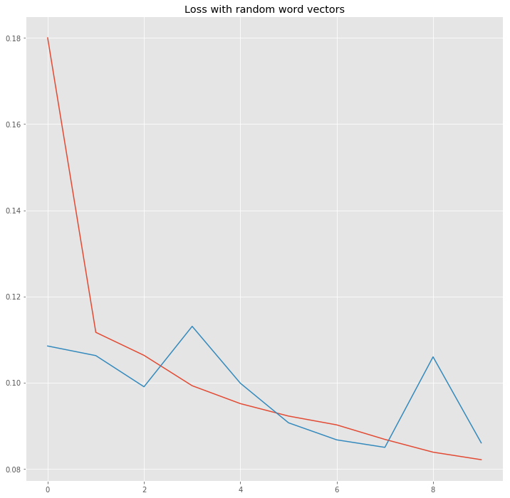
We see the loss decreasing much slower and the validation loss is pretty unstable.
I hope you enjoyed this post and it is useful to you. Have fun with word vectors!