This is the fourth post in my series about named entity recognition. If you haven’t seen the last three, have a look now. The last time we used a recurrent neural network to model the sequence structure of our sentences. Now we use a hybrid approach combining a bidirectional LSTM model and a CRF model. This is a state-of-the-art approach to named entity recognition.
Let’s recall the situation from the article about conditional random fields. We are given a input sequence $x = (x_1,\dots, x_m)$, i.e. the words of a sentence and a sequence of output states $s = (s_1,\dots, s_m)$, i.e. the named entity tags. In conditional random fields we modeled the conditional probability $$p(s_1,\dots,s_m|x_1,\dots,x_m)$$ of the output state sequence give a input sequence. We did this by defining a feature map $$\Phi(x_1,\dots,x_m,s_1,\dots,s_m)\in\mathbb{R}^d$$ that maps an entire input sequence $x$ paired with an entire state sequence $s$ to some $d$-dimensional feature vector. Then we can model the probability as a log-linear model with the parameter vector $w\in\mathbb{R}^d$ $$p(s|x; w) = \frac{\exp(w\cdot\Phi(x, s))}{\sum_{s^\prime} \exp(w\cdot\Phi(x, s^\prime))},$$ where $s^\prime$ ranges over all possible output sequences. We can view the expression $w\cdot\Phi(x, s) = \text{score}_{crf}(x,s)$ as a scoring how well the state sequence fits the given input sequence. The idea is now, to replace the linear scoring function by a non-linear neural network. So we define the score $$\text{score}_{lstm-crf}(x,s) = \sum_{i=0}^n W_{s_{i-1}, s_i} \cdot \text{LSTM}(x)_i + b_{s_{i-1},s_i},$$ where $W_{s_{i-1}, s_i}$ and $b$ are the weight vector and the bias corresponding to the transition from $s_{i-1}$ to $s_i$, respectively. Note, that the score functions are also called $\textit{potential functions}$. After constructing this score function, we can optimize the conditional probability $p(s|x; W, b)$ like in the usual CRF and propagating back trough the network. We are going to use the implementation provided by the keras-contrib package, that contains useful extensions to the official keras package.
Load the data
Now dive into the applied part. We start as always by loading the data. If you want to run the tutorial yourself, you can find the dataset here.
import pandas as pd
import numpy as np

data = pd.read_csv("ner_dataset.csv", encoding="latin1")
data = data.fillna(method="ffill")
data.tail(10)
| Sentence # | Word | POS | Tag | |
|---|---|---|---|---|
| 1048565 | Sentence: 47958 | impact | NN | O |
| 1048566 | Sentence: 47958 | . | . | O |
| 1048567 | Sentence: 47959 | Indian | JJ | B-gpe |
| 1048568 | Sentence: 47959 | forces | NNS | O |
| 1048569 | Sentence: 47959 | said | VBD | O |
| 1048570 | Sentence: 47959 | they | PRP | O |
| 1048571 | Sentence: 47959 | responded | VBD | O |
| 1048572 | Sentence: 47959 | to | TO | O |
| 1048573 | Sentence: 47959 | the | DT | O |
| 1048574 | Sentence: 47959 | attack | NN | O |
words = list(set(data["Word"].values))
words.append("ENDPAD")
n_words = len(words); n_words
35179
tags = list(set(data["Tag"].values))
n_tags = len(tags); n_tags
17
So we have 47959 sentences containing 35178 different words with 17 different tags. We use the SentenceGetter class from last post to retrieve sentences with their labels.
class SentenceGetter(object):

    def __init__(self, data):
        self.n_sent = 1
        self.data = data
        self.empty = False
        agg_func = lambda s: [(w, p, t) for w, p, t in zip(s["Word"].values.tolist(),
                                                           s["POS"].values.tolist(),
                                                           s["Tag"].values.tolist())]
        self.grouped = self.data.groupby("Sentence #").apply(agg_func)
        self.sentences = [s for s in self.grouped]

    def get_next(self):
        try:
            s = self.grouped["Sentence: {}".format(self.n_sent)]
            self.n_sent += 1
            return s
        except:
            return None
getter = SentenceGetter(data)
sent = getter.get_next()
This is how a sentence looks now.
print(sent)
[('Thousands', 'NNS', 'O'), ('of', 'IN', 'O'), ('demonstrators', 'NNS', 'O'), ('have', 'VBP', 'O'), ('marched', 'VBN', 'O'), ('through', 'IN', 'O'), ('London', 'NNP', 'B-geo'), ('to', 'TO', 'O'), ('protest', 'VB', 'O'), ('the', 'DT', 'O'), ('war', 'NN', 'O'), ('in', 'IN', 'O'), ('Iraq', 'NNP', 'B-geo'), ('and', 'CC', 'O'), ('demand', 'VB', 'O'), ('the', 'DT', 'O'), ('withdrawal', 'NN', 'O'), ('of', 'IN', 'O'), ('British', 'JJ', 'B-gpe'), ('troops', 'NNS', 'O'), ('from', 'IN', 'O'), ('that', 'DT', 'O'), ('country', 'NN', 'O'), ('.', '.', 'O')]
Okay, that looks like expected, now get all sentences.
sentences = getter.sentences
Now we introduce dictionaries of words and tags.
max_len = 75
word2idx = {w: i + 1 for i, w in enumerate(words)}
tag2idx = {t: i for i, t in enumerate(tags)}
word2idx["Obama"]
21474
tag2idx["B-geo"]
5
Tokenize and prepare the sentences
Now we map the sentences to a sequence of numbers and then pad the sequence. Note that we increased the index of the words by one to use zero as a padding value. This is done because we want to use the mask_zero parameter of the embedding layer to ignore inputs with value zero.
from keras.preprocessing.sequence import pad_sequences
X = [[word2idx[w[0]] for w in s] for s in sentences]
Using TensorFlow backend.
X = pad_sequences(maxlen=max_len, sequences=X, padding="post", value=0)
And we need to do the same for our tag sequence.
y = [[tag2idx[w[2]] for w in s] for s in sentences]
y = pad_sequences(maxlen=max_len, sequences=y, padding="post", value=tag2idx["O"])
For training the network we also need to change the labels $y$ to categorial.
from keras.utils import to_categorical
y = [to_categorical(i, num_classes=n_tags) for i in y]
We split in train and test set.
from sklearn.model_selection import train_test_split
X_tr, X_te, y_tr, y_te = train_test_split(X, y, test_size=0.1)
Train the model
Now we can fit a LSTM-CRF network with an embedding layer.
from keras.models import Model, Input
from keras.layers import LSTM, Embedding, Dense, TimeDistributed, Dropout, Bidirectional
from keras_contrib.layers import CRF
input = Input(shape=(max_len,))
model = Embedding(input_dim=n_words + 1, output_dim=20,
                  input_length=max_len, mask_zero=True)(input)  # 20-dim embedding
model = Bidirectional(LSTM(units=50, return_sequences=True,
                           recurrent_dropout=0.1))(model)  # variational biLSTM
model = TimeDistributed(Dense(50, activation="relu"))(model)  # a dense layer as suggested by neuralNer
crf = CRF(n_tags)  # CRF layer
out = crf(model)  # output
model = Model(input, out)
model.compile(optimizer="rmsprop", loss=crf.loss_function, metrics=[crf.accuracy])
model.summary()
_________________________________________________________________
Layer (type)                 Output Shape              Param #
=================================================================
input_1 (InputLayer)         (None, 75)                0
_________________________________________________________________
embedding_1 (Embedding)      (None, 75, 20)            703600
_________________________________________________________________
bidirectional_1 (Bidirection (None, 75, 100)           28400
_________________________________________________________________
time_distributed_1 (TimeDist (None, 75, 50)            5050
_________________________________________________________________
crf_1 (CRF)                  (None, 75, 17)            1190
=================================================================
Total params: 738,240
Trainable params: 738,240
Non-trainable params: 0
_________________________________________________________________
history = model.fit(X_tr, np.array(y_tr), batch_size=32, epochs=5,
                    validation_split=0.1, verbose=1)
Train on 38846 samples, validate on 4317 samples
Epoch 1/5
38846/38846 [==============================] - 333s 9ms/step - loss: 8.8985 - acc: 0.9030 - val_loss: 8.8571 - val_acc: 0.9515
Epoch 2/5
38846/38846 [==============================] - 331s 9ms/step - loss: 8.6684 - acc: 0.9603 - val_loss: 8.8104 - val_acc: 0.9636
Epoch 3/5
38846/38846 [==============================] - 331s 9ms/step - loss: 8.6415 - acc: 0.9676 - val_loss: 8.7996 - val_acc: 0.9661
Epoch 4/5
38846/38846 [==============================] - 332s 9ms/step - loss: 8.6312 - acc: 0.9704 - val_loss: 8.7952 - val_acc: 0.9674
Epoch 5/5
38846/38846 [==============================] - 331s 9ms/step - loss: 8.6250 - acc: 0.9724 - val_loss: 8.7930 - val_acc: 0.9677
hist = pd.DataFrame(history.history)
import matplotlib.pyplot as plt
plt.style.use("ggplot")
plt.figure(figsize=(12, 12))
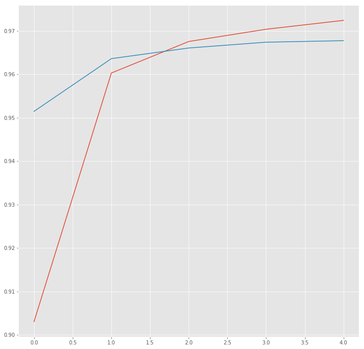
plt.plot(hist["acc"])
plt.plot(hist["val_acc"])
plt.show()
Evaluate
Now we can evaluate our model systematically. You can find the details in this post, here we just apply it.
from seqeval.metrics import precision_score, recall_score, f1_score, classification_report
test_pred = model.predict(X_te, verbose=1)
4796/4796 [==============================] - 11s 2ms/step
idx2tag = {i: w for w, i in tag2idx.items()}

def pred2label(pred):
    out = []
    for pred_i in pred:
        out_i = []
        for p in pred_i:
            p_i = np.argmax(p)
            out_i.append(idx2tag[p_i].replace("PAD", "O"))
        out.append(out_i)
    return out

pred_labels = pred2label(test_pred)
test_labels = pred2label(y_te)
print("F1-score: {:.1%}".format(f1_score(test_labels, pred_labels)))
F1-score: 67.1%
print(classification_report(test_labels, pred_labels))
             precision    recall  f1-score   support

        geo       0.84      0.88      0.86      3603
        per       0.77      0.76      0.77      1734
        gpe       0.97      0.91      0.94      1520
        tim       0.90      0.84      0.87      2013
        org       0.70      0.66      0.68      1988
        eve       0.50      0.03      0.05        37
        nat       0.00      0.00      0.00        14
        art       0.00      0.00      0.00        49

avg / total       0.83      0.81      0.82     10958
Finally, we look at some predictions.
i = 1928
p = model.predict(np.array([X_te[i]]))
p = np.argmax(p, axis=-1)
true = np.argmax(y_te[i], -1)
print("{:15}||{:5}||{}".format("Word", "True", "Pred"))
print(30 * "=")
for w, t, pred in zip(X_te[i], true, p[0]):
    if w != 0:
        print("{:15}: {:5} {}".format(words[w-1], tags[t], tags[pred]))
This looks pretty good and it did require any feature engineering. The power of the CRF is not really visible here, but if we had a dataset with more complicated named entities this would be quite strong.
Predict on new data
UPDATE: Since many people asked how to use this with new data, which is obviously important, I show you now how to do it. To stay in the frame of this tutorial, I will assume the text is already tokenized. If you don’t know how to do this, I recommend looking at my post about word vectors.
test_sentence = ["Hawking", "was", "a", "Fellow", "of", "the", "Royal", "Society", ",", "a", "lifetime", "member",
                 "of", "the", "Pontifical", "Academy", "of", "Sciences", ",", "and", "a", "recipient", "of",
                 "the", "Presidential", "Medal", "of", "Freedom", ",", "the", "highest", "civilian", "award",
                 "in", "the", "United", "States", "."]
Now we transform every word to it’s integer index. Note that we mapping unknown words to zero. Normally you would want to add a UNKNOWN token to your vocabulary. Then you cut the vocabulary on which you train the model and replace all uncommon words by the UNKNOWN token. We haven’t done this for simplicity.
x_test_sent = pad_sequences(sequences=[[word2idx.get(w, 0) for w in test_sentence]],
                            padding="post", value=0, maxlen=max_len)
And now we can predict with the model and see what we got.
tags
p = model.predict(np.array([x_test_sent[0]]))
p = np.argmax(p, axis=-1)
print("{:15}||{}".format("Word", "Prediction"))
print(30 * "=")
for w, pred in zip(test_sentence, p[0]):
    print("{:15}: {:5}".format(w, tags[pred]))
I hope you enjoyed this post and learned something that you can apply in your daily work. Next time I show you how you can improve the model even further by using character-level embeddings.
References and further reading:
- Z. Huang et. al Bidirectional LSTM-CRF Models for Sequence Tagging
- X. Ma et al. End-to-end Sequence Labeling via Bi-directional LSTM-CNNs-CRF