In this article, we will apply the concept of multi-label multi-class classification with neural networks from the last post, to classify movie posters by genre. First we import the usual suspects in python.
import numpy as np
import pandas as pd
import glob
import scipy.misc
import matplotlib
%matplotlib inline
import matplotlib.pyplot as plt
…and then we import the movie metadata.
path = 'posters/'
data = pd.read_csv("MovieGenre.csv", encoding="ISO-8859-1")
Now have a look at it.
data.head()
| imdbId | Imdb Link | Title | IMDB Score | Genre | Poster | |
|---|---|---|---|---|---|---|
| 0 | 114709 | http://www.imdb.com/title/tt114709 | Toy Story (1995) | 8.3 | Animation|Adventure|Comedy | https://images-na.ssl-images-amazon.com/images... |
| 1 | 113497 | http://www.imdb.com/title/tt113497 | Jumanji (1995) | 6.9 | Action|Adventure|Family | https://images-na.ssl-images-amazon.com/images... |
| 2 | 113228 | http://www.imdb.com/title/tt113228 | Grumpier Old Men (1995) | 6.6 | Comedy|Romance | https://images-na.ssl-images-amazon.com/images... |
| 3 | 114885 | http://www.imdb.com/title/tt114885 | Waiting to Exhale (1995) | 5.7 | Comedy|Drama|Romance | https://images-na.ssl-images-amazon.com/images... |
| 4 | 113041 | http://www.imdb.com/title/tt113041 | Father of the Bride Part II (1995) | 5.9 | Comedy|Family|Romance | https://images-na.ssl-images-amazon.com/images... |
Next, we load the movie posters.
image_glob = glob.glob(path + "/" + "*.jpg")
img_dict = {}


def get_id(filename):
    index_s = filename.rfind("/") + 1
    index_f = filename.rfind(".jpg")
    return filename[index_s:index_f]
for fn in image_glob:
    try:
        img_dict[get_id(fn)] = scipy.misc.imread(fn)
    except:
        pass
def show_img(id):
    title = data[data["imdbId"] == int(id)]["Title"].values[0]
    genre = data[data["imdbId"] == int(id)]["Genre"].values[0]
    plt.imshow(img_dict[id])
    plt.title("{} \n {}".format(title, genre))
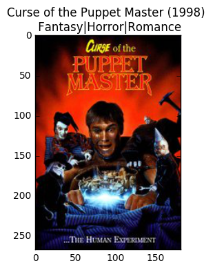
Let’s look at an example:
show_img("3405714")
Now we start the modelling.
For this we write a neat little preprocessing function to scale the image…
def preprocess(img, size=(150, 101)):
    img = scipy.misc.imresize(img, size)
    img = img.astype(np.float32)
    img = (img / 127.5) - 1.
    return img
… and a function to generate our data set.
def prepare_data(data, img_dict, size=(150, 101)):
    print("Generation dataset...")
    dataset = []
    y = []
    ids = []
    label_dict = {"word2idx": {}, "idx2word": []}
    idx = 0
    genre_per_movie = data["Genre"].apply(lambda x: str(x).split("|"))
    for l in [g for d in genre_per_movie for g in d]:
        if l in label_dict["idx2word"]:
            pass
        else:
            label_dict["idx2word"].append(l)
            label_dict["word2idx"][l] = idx
            idx += 1
    n_classes = len(label_dict["idx2word"])
    print("identified {} classes".format(n_classes))
    n_samples = len(img_dict)
    print("got {} samples".format(n_samples))
    for k in img_dict:
        try:
            g = data[data["imdbId"] == int(k)]["Genre"].values[0].split("|")
            img = preprocess(img_dict[k], size)
            if img.shape != (150, 101, 3):
                continue
            l = np.sum([np.eye(n_classes, dtype="uint8")[label_dict["word2idx"][s]] for s in g], axis=0)
            y.append(l)
            dataset.append(img)
            ids.append(k)
        except:
            pass
    print("DONE")
    return dataset, y, label_dict, ids
We scale our movie posters to 96x96.
SIZE = (150, 101)
dataset, y, label_dict, ids =  prepare_data(data, img_dict, size=SIZE)
Generation dataset...
identified 29 classes
got 38667 samples
DONE
Now we build the model. We start with a small VGG-like convolutional neural net.
import keras
from keras.models import Sequential
from keras.layers import Dense, Dropout, Flatten
from keras.layers import Conv2D, MaxPooling2D, BatchNormalization
model = Sequential()
model.add(Conv2D(32, kernel_size=(3, 3), activation='relu', input_shape=(SIZE[0], SIZE[1], 3)))
model.add(Conv2D(32, (3, 3), activation='relu'))
model.add(MaxPooling2D(pool_size=(2, 2)))
model.add(Dropout(0.25))

model.add(Conv2D(64, kernel_size=(3, 3), activation='relu'))
model.add(Conv2D(64, (3, 3), activation='relu'))
model.add(MaxPooling2D(pool_size=(2, 2)))
model.add(Dropout(0.25))

model.add(Flatten())
model.add(Dense(128, activation='relu'))
model.add(Dropout(0.5))
model.add(Dense(29, activation='sigmoid'))
It’s important to notice, that we use a sigmoid activation function with a multiclass output-layer. The sigmoid gives us independent probabilities for each class. So DON’T use softmax here!
model.compile(loss='binary_crossentropy',
              optimizer=keras.optimizers.Adam(),
              metrics=['accuracy'])
n = 10000
model.fit(np.array(dataset[: n]), np.array(y[: n]), batch_size=16, epochs=5,
          verbose=1, validation_split=0.1)
Train on 9000 samples, validate on 1000 samples
Epoch 1/5
9000/9000 [==============================] - 900s - loss: 0.2352 - acc: 0.9194 - val_loss: 0.2022 - val_acc: 0.9278
Epoch 2/5
9000/9000 [==============================] - 904s - loss: 0.2123 - acc: 0.9260 - val_loss: 0.2016 - val_acc: 0.9279
Epoch 3/5
9000/9000 [==============================] - 854s - loss: 0.2083 - acc: 0.9268 - val_loss: 0.2007 - val_acc: 0.9286
Epoch 4/5
9000/9000 [==============================] - 887s - loss: 0.2058 - acc: 0.9274 - val_loss: 0.2023 - val_acc: 0.9294
Epoch 5/5
9000/9000 [==============================] - 944s - loss: 0.2031 - acc: 0.9282 - val_loss: 0.1991 - val_acc: 0.9289


<keras.callbacks.History at 0x7f08b8cebd68>
Let’s predict…
n_test = 100
X_test = dataset[n:n + n_test]
y_test = y[n:n + n_test]
pred = model.predict(np.array(X_test))
… and look at a few samples.
def show_example(idx):
    N_true = int(np.sum(y_test[idx]))
    show_img(ids[n + idx])
    print("Prediction: {}".format("|".join(["{} ({:.3})".format(label_dict["idx2word"][s], pred[idx][s])
                                            for s in pred[idx].argsort()[-N_true:][::-1]])))
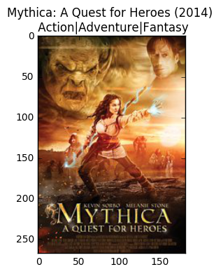
show_example(3)
Prediction: Drama (0.496)|Horror (0.203)|Thriller (0.182)
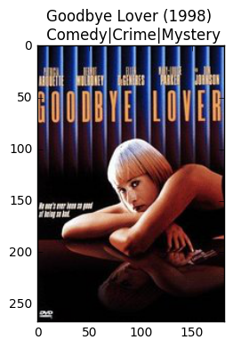
show_example(97)
Prediction: Drama (0.509)|Comedy (0.371)|Romance (0.217)
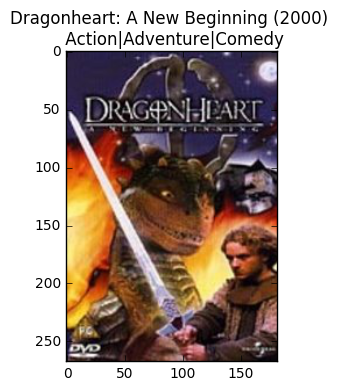
show_example(48)
Prediction: Drama (0.453)|Comedy (0.277)|Horror (0.19)
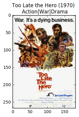
show_example(68)
Prediction: Drama (0.474)|Horror (0.245)|Thriller (0.227)
This looks pretty interesting, but not very good. It always predicts “Drama”. I think this is because it is the most common genre in the dataset. We could overcome this by using a class weight. We could now try to increase the number of training samples, try a different network architecture or just train longer.