Deep learning models have shown amazing performance in a lot of fields such as autonomous driving, manufacturing, and medicine, to name a few. However, these are fields in which representing model uncertainty is of crucial importance. The standard deep learning tools for regression and classification do not capture model uncertainty. In classification, predictive probabilities obtained at the end of the pipeline (the softmax output) are often erroneously interpreted as model confidence. Gal et. al argue, that a model can be uncertain in its predictions even with a high softmax output. Passing a point estimate of a function through a softmax results in extrapolations with unjustified high confidence for points far from the training data.
Model uncertainty is indispensable for the deep learning practitioner as well. With model confidence at hand we can treat uncertain inputs and special cases explicitly. I recommend Vincents talk from pydata london for a general view on the topic. For example, in the case of classification, a model might return a result with high uncertainty. In this case we might decide to pass the input to a human for classification.
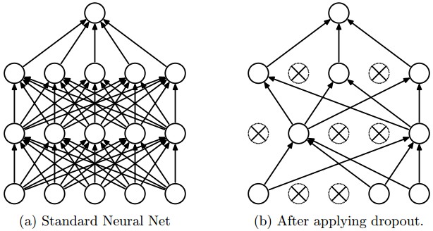
Gal et. al show that the use of dropout in neural networks can be interpreted as a Bayesian approximation of a Gaussian process, a well known probabilistic model. Dropout is used in many models in deep learning as a way to avoid over-fitting, and they show that dropout approximately integrates over the models’ weights. In this article we will see how to represent model uncertainty of existing dropout neural networks. This approach, called Monte Carlo dropout, will mitigates the problem of representing model uncertainty in deep learning without sacrificing either computational complexity or test accuracy and can be used for all kind of models trained with dropout.
Load the MNIST data
We will use the MNIST dataset to explore the proposed method of Monte Carlo dropout. We can conveniently load it with keras.
from __future__ import print_function
import keras
from keras.datasets import mnist
from keras.models import Sequential, Model, Input
from keras.layers import Dense, Dropout, Flatten, SpatialDropout2D, SpatialDropout1D, AlphaDropout
from keras.layers import Conv2D, MaxPooling2D
from keras import backend as K

import numpy as np
import pandas as pd
from sklearn.metrics import accuracy_score

import matplotlib.pyplot as plt
plt.style.use("ggplot")
%matplotlib inline
Using TensorFlow backend.
batch_size = 128
num_classes = 10
epochs = 12

# input image dimensions
img_rows, img_cols = 28, 28
# the data, split between train and test sets
(x_train, y_train), (x_test, y_test) = mnist.load_data()
if K.image_data_format() == 'channels_first':
    x_train = x_train.reshape(x_train.shape[0], 1, img_rows, img_cols)
    x_test = x_test.reshape(x_test.shape[0], 1, img_rows, img_cols)
    input_shape = (1, img_rows, img_cols)
else:
    x_train = x_train.reshape(x_train.shape[0], img_rows, img_cols, 1)
    x_test = x_test.reshape(x_test.shape[0], img_rows, img_cols, 1)
    input_shape = (img_rows, img_cols, 1)
x_train = x_train.astype('float32')
x_test = x_test.astype('float32')
x_train /= 255
x_test /= 255
print('x_train shape:', x_train.shape)
print(x_train.shape[0], 'train samples')
print(x_test.shape[0], 'test samples')
x_train shape: (60000, 28, 28, 1)
60000 train samples
10000 test samples
# convert class vectors to binary class matrices
y_train = keras.utils.to_categorical(y_train, num_classes)
y_test = keras.utils.to_categorical(y_test, num_classes)
Build Monte Carlo Model and run experiments
Modeling uncertainty with Monte Carlo dropout works by running multiple forward passes trough the model with a different dropout masks every time. Let’s say we are given a trained neural network model with dropout $f_{nn}$. To derive the uncertainty for one sample $x$ we collect the predictions of $T$ inferences with different dropout masks. Here $f_{nn}^{d_i}$ represents the model with dropout mask $d_i$. So we obtain a sample of the possible model outputs for sample $x$ as $${f_{nn}^{d_0}(x), \dots, f_{nn}^{d_T}(x)}.$$ By computing the average and the variance of this sample we get an ensemble prediction, which is the mean of the models posterior distribution for this sample and an estimate of the uncertainty of the model regarding $x$. $$\text{predictive posterior mean:}\quad p = \frac{1}{T} \sum_{i=0}^T f_{nn}^{d_i}(x)$$ $$\text{uncertainty:}\quad c = \frac{1}{T} \sum_{i=0}^T \left[f_{nn}^{d_i}(x) - p\right]^2$$
Note that the dropout NN model itself is not changed. To estimate the predictive mean and predictive uncertainty we simply collect the results of stochastic forward passes through the model. As a result, this information can be used with existing NN models trained with dropout.
To achieve this in keras, we have to use the functional API and setup dropout this way: Dropout(p)(input_tensor, training=True). We build a simple convolutional network with a without Monte Carlo dropout and compare their properties.
def get_dropout(input_tensor, p=0.5, mc=False):
    if mc:
        return Dropout(p)(input_tensor, training=True)
    else:
        return Dropout(p)(input_tensor)


def get_model(mc=False, act="relu"):
    inp = Input(input_shape)
    x = Conv2D(32, kernel_size=(3, 3), activation=act)(inp)
    x = Conv2D(64, kernel_size=(3, 3), activation=act)(x)
    x = MaxPooling2D(pool_size=(2, 2))(x)
    x = get_dropout(x, p=0.25, mc=mc)
    x = Flatten()(x)
    x = Dense(128, activation=act)(x)
    x = get_dropout(x, p=0.5, mc=mc)
    out = Dense(num_classes, activation='softmax')(x)

    model = Model(inputs=inp, outputs=out)

    model.compile(loss=keras.losses.categorical_crossentropy,
                  optimizer=keras.optimizers.Adadelta(),
                  metrics=['accuracy'])
    return model
model = get_model(mc=False, act="relu")
mc_model = get_model(mc=True, act="relu")
h = model.fit(x_train, y_train,
              batch_size=batch_size,
              epochs=10,
              verbose=1,
              validation_data=(x_test, y_test))
Train on 60000 samples, validate on 10000 samples
Epoch 1/10
60000/60000 [==============================] - 48s 802us/step - loss: 0.2599 - acc: 0.9217 - val_loss: 0.0555 - val_acc: 0.9832
Epoch 2/10
60000/60000 [==============================] - 47s 779us/step - loss: 0.0871 - acc: 0.9746 - val_loss: 0.0401 - val_acc: 0.9861
Epoch 3/10
60000/60000 [==============================] - 47s 781us/step - loss: 0.0642 - acc: 0.9807 - val_loss: 0.0329 - val_acc: 0.9876
Epoch 4/10
60000/60000 [==============================] - 47s 780us/step - loss: 0.0524 - acc: 0.9845 - val_loss: 0.0312 - val_acc: 0.9896
Epoch 5/10
60000/60000 [==============================] - 47s 780us/step - loss: 0.0467 - acc: 0.9860 - val_loss: 0.0308 - val_acc: 0.9903
Epoch 6/10
60000/60000 [==============================] - 47s 781us/step - loss: 0.0409 - acc: 0.9873 - val_loss: 0.0254 - val_acc: 0.9918
Epoch 7/10
60000/60000 [==============================] - 47s 780us/step - loss: 0.0373 - acc: 0.9887 - val_loss: 0.0277 - val_acc: 0.9906
Epoch 8/10
60000/60000 [==============================] - 47s 781us/step - loss: 0.0343 - acc: 0.9896 - val_loss: 0.0265 - val_acc: 0.9916
Epoch 9/10
60000/60000 [==============================] - 47s 783us/step - loss: 0.0309 - acc: 0.9907 - val_loss: 0.0253 - val_acc: 0.9921
Epoch 10/10
60000/60000 [==============================] - 47s 781us/step - loss: 0.0302 - acc: 0.9907 - val_loss: 0.0298 - val_acc: 0.9914
# score of the normal model
score = model.evaluate(x_test, y_test, verbose=0)

print('Test loss:', score[0])
print('Test accuracy:', score[1])
Test loss: 0.029758870216909507
Test accuracy: 0.9914
h_mc = mc_model.fit(x_train, y_train,
                    batch_size=batch_size,
                    epochs=10,
                    verbose=1,
                    validation_data=(x_test, y_test))
Train on 60000 samples, validate on 10000 samples
Epoch 1/10
60000/60000 [==============================] - 48s 793us/step - loss: 0.2621 - acc: 0.9196 - val_loss: 0.0994 - val_acc: 0.9725
Epoch 2/10
60000/60000 [==============================] - 46s 774us/step - loss: 0.0878 - acc: 0.9732 - val_loss: 0.0713 - val_acc: 0.9776
Epoch 3/10
60000/60000 [==============================] - 46s 774us/step - loss: 0.0665 - acc: 0.9805 - val_loss: 0.0559 - val_acc: 0.9818
Epoch 4/10
60000/60000 [==============================] - 47s 777us/step - loss: 0.0554 - acc: 0.9842 - val_loss: 0.0554 - val_acc: 0.9839
Epoch 5/10
60000/60000 [==============================] - 47s 777us/step - loss: 0.0466 - acc: 0.9860 - val_loss: 0.0526 - val_acc: 0.9835
Epoch 6/10
60000/60000 [==============================] - 46s 775us/step - loss: 0.0406 - acc: 0.9878 - val_loss: 0.0497 - val_acc: 0.9843
Epoch 7/10
60000/60000 [==============================] - 46s 774us/step - loss: 0.0369 - acc: 0.9889 - val_loss: 0.0483 - val_acc: 0.9844
Epoch 8/10
60000/60000 [==============================] - 47s 776us/step - loss: 0.0335 - acc: 0.9901 - val_loss: 0.0478 - val_acc: 0.9858
Epoch 9/10
60000/60000 [==============================] - 47s 776us/step - loss: 0.0316 - acc: 0.9898 - val_loss: 0.0418 - val_acc: 0.9872
Epoch 10/10
60000/60000 [==============================] - 47s 778us/step - loss: 0.0294 - acc: 0.9910 - val_loss: 0.0481 - val_acc: 0.9850
import tqdm

mc_predictions = []
for i in tqdm.tqdm(range(500)):
    y_p = mc_model.predict(x_test, batch_size=1000)
    mc_predictions.append(y_p)
100%|██████████| 500/500 [17:02<00:00, 2.04s/it]
# score of the mc model
accs = []
for y_p in mc_predictions:
    acc = accuracy_score(y_test.argmax(axis=1), y_p.argmax(axis=1))
    accs.append(acc)
print("MC accuracy: {:.1%}".format(sum(accs)/len(accs)))
MC accuracy: 98.6%
mc_ensemble_pred = np.array(mc_predictions).mean(axis=0).argmax(axis=1)
ensemble_acc = accuracy_score(y_test.argmax(axis=1), mc_ensemble_pred)
print("MC-ensemble accuracy: {:.1%}".format(ensemble_acc))
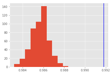
MC-ensemble accuracy: 99.2%
Look at the distributions of the monte carlo predictions and in blue you see the prediction of the ensemble.
plt.hist(accs);
plt.axvline(x=ensemble_acc, color="b");
Explore the Monte Carlo predictions
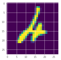
We look at images and their assigned predictions with probability and uncertainty.
idx = 247
plt.imshow(x_test[idx][:,:,0])
<matplotlib.image.AxesImage at 0x7fa9ad2d5b38>
p0 = np.array([p[idx] for p in mc_predictions])
print("posterior mean: {}".format(p0.mean(axis=0).argmax()))
print("true label: {}".format(y_test[idx].argmax()))
print()
# probability + variance
for i, (prob, var) in enumerate(zip(p0.mean(axis=0), p0.std(axis=0))):
    print("class: {}; proba: {:.1%}; var: {:.2%} ".format(i, prob, var))
posterior mean: 4
true label: 4

class: 0; proba: 0.0%; var: 0.20%
class: 1; proba: 9.8%; var: 19.46%
class: 2; proba: 12.5%; var: 22.34%
class: 3; proba: 0.0%; var: 0.01%
class: 4; proba: 56.0%; var: 34.90%
class: 5; proba: 0.1%; var: 1.17%
class: 6; proba: 21.0%; var: 28.19%
class: 7; proba: 0.1%; var: 1.67%
class: 8; proba: 0.5%; var: 4.71%
class: 9; proba: 0.0%; var: 0.02%
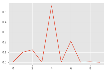
x, y = list(range(len(p0.mean(axis=0)))), p0.mean(axis=0)
plt.plot(x, y);
fig, axes = plt.subplots(5, 2, figsize=(12,12))

for i, ax in enumerate(fig.get_axes()):
    ax.hist(p0[:,i], bins=100, range=(0,1));
    ax.set_title(f"class {i}")
    ax.label_outer()
We see, that the model is correct but fairly uncertain. This seems to be a hard example. We would probably let a human decide what to do with this example.
Find the most uncertain examples
Next, we find the most uncertain examples. This can be useful to understand your dataset or where the model has problems.
1. Selection by probability
First we select images by the predictive mean, our probability.
max_means = []
preds = []
for idx in range(len(mc_predictions)):
    px = np.array([p[idx] for p in mc_predictions])
    preds.append(px.mean(axis=0).argmax())
    max_means.append(px.mean(axis=0).max())
(np.array(max_means)).argsort()[:10]
array([247, 175, 115, 445, 340, 320, 62, 321, 259, 449])
plt.imshow(x_test[247][:,:,0])
<matplotlib.image.AxesImage at 0x7fa9ad1f7eb8>

It seems the image from above was the one the model was most uncertain about by probability.
2. Selection by variance
Now we can select the images by the variance of the predictions.
max_vars = []
for idx in range(len(mc_predictions)):
    px = np.array([p[idx] for p in mc_predictions])
    max_vars.append(px.std(axis=0)[px.mean(axis=0).argmax()])
(-np.array(max_vars)).argsort()[:10]
array([247, 259, 62, 449, 115, 320, 445, 492, 211, 326])
plt.imshow(x_test[259][:,:,0])
<matplotlib.image.AxesImage at 0x7fa9af4fb3c8>
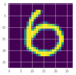
How is the uncertainty measure behaved?
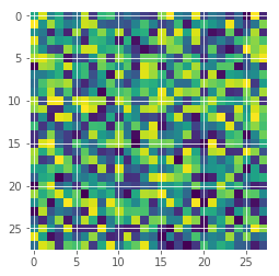
One important test is how well can the uncertainty estimate identify out-of-scope samples. Here we just create random images and see what the model predicts.
random_img = np.random.random(input_shape)
plt.imshow(random_img[:,:,0]);
random_predictions = []
for i in tqdm.tqdm(range(500)):
    y_p = mc_model.predict(np.array([random_img]))
    random_predictions.append(y_p)
100%|██████████| 500/500 [00:01<00:00, 258.86it/s]
p0 = np.array([p[0] for p in random_predictions])
print("posterior mean: {}".format(p0.mean(axis=0).argmax()))
print()
# probability + variance
for i, (prob, var) in enumerate(zip(p0.mean(axis=0), p0.std(axis=0))):
    print("class: {}; proba: {:.1%}; var: {:.2%} ".format(i, prob, var))
posterior mean: 8

class: 0; proba: 1.8%; var: 2.03%
class: 1; proba: 0.7%; var: 1.24%
class: 2; proba: 4.7%; var: 4.87%
class: 3; proba: 8.8%; var: 8.90%
class: 4; proba: 1.1%; var: 2.25%
class: 5; proba: 4.6%; var: 6.50%
class: 6; proba: 1.5%; var: 1.83%
class: 7; proba: 0.2%; var: 0.51%
class: 8; proba: 76.1%; var: 14.25%
class: 9; proba: 0.5%; var: 1.08%
x, y = list(range(len(p0.mean(axis=0)))), p0.mean(axis=0)
plt.plot(x, y);
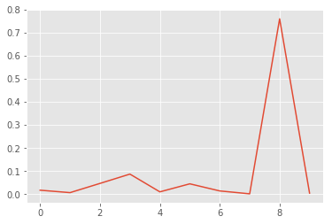
Wow, this is bad! The model is pretty certain that this is an eight. But it is clearly just random noise. If you try different random images, you will find that the model always predicts them as eight. So there might be something wrong with the “understanding” of eight in our model. This is good to know and keep in mind when using the model.
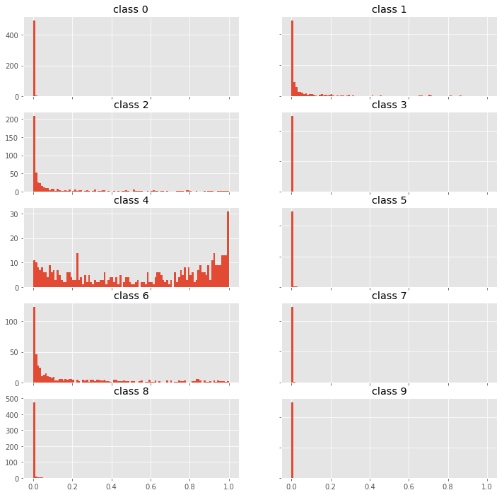
fig, axes = plt.subplots(5, 2, figsize=(12,12))

for i, ax in enumerate(fig.get_axes()):
    ax.hist(p0[:,i], bins=100, range=(0,1));
    ax.set_title(f"class {i}")
    ax.label_outer()
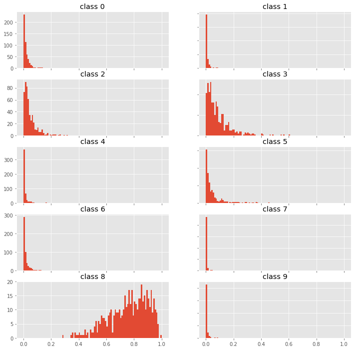
Looking at the probability distributions of the predictions for different classes we can probably find a way to identify out-of-scope samples by using higher moments than just mean and variance. Try it and let me know what you find.
That’s all for now. We saw a simple but effective way to derive uncertainty estimates for deep learning models, a useful tool in your machine learning toolbox. I hope you liked this tutorial and it will be helpful to you. Watch out for more to come on this topic!