This is the third post in my series about named entity recognition. If you haven’t seen the last two, have a look now. The last time we used a conditional random field to model the sequence structure of our sentences. This time we use a LSTM model to do the tagging. At the end of this guide, you will know how to use neural networks to tag sequences of words. For more details on neural nets and LSTM in particular, I suggest to read this excellent post.
Load the data
Now we want to apply this model. Let’s start by loading the data. If you want to run the tutorial yourself, you can find the dataset here.
import pandas as pd
import numpy as np

data = pd.read_csv("ner_dataset.csv", encoding="latin1")
data = data.fillna(method="ffill")
data.tail(10)
| Sentence # | Word | POS | Tag | |
|---|---|---|---|---|
| 1048565 | Sentence: 47958 | impact | NN | O |
| 1048566 | Sentence: 47958 | . | . | O |
| 1048567 | Sentence: 47959 | Indian | JJ | B-gpe |
| 1048568 | Sentence: 47959 | forces | NNS | O |
| 1048569 | Sentence: 47959 | said | VBD | O |
| 1048570 | Sentence: 47959 | they | PRP | O |
| 1048571 | Sentence: 47959 | responded | VBD | O |
| 1048572 | Sentence: 47959 | to | TO | O |
| 1048573 | Sentence: 47959 | the | DT | O |
| 1048574 | Sentence: 47959 | attack | NN | O |
Prepare the dataset
words = list(set(data["Word"].values))
words.append("ENDPAD")
n_words = len(words); n_words
35179
tags = list(set(data["Tag"].values))
n_tags = len(tags); n_tags
17
So we have 47959 sentences containing 35178 different words with 17 different tags. We use the SentenceGetter class from last post to retrieve sentences with their labels.
class SentenceGetter(object):

    def __init__(self, data):
        self.n_sent = 1
        self.data = data
        self.empty = False
        agg_func = lambda s: [(w, p, t) for w, p, t in zip(s["Word"].values.tolist(),
                                                           s["POS"].values.tolist(),
                                                           s["Tag"].values.tolist())]
        self.grouped = self.data.groupby("Sentence #").apply(agg_func)
        self.sentences = [s for s in self.grouped]

    def get_next(self):
        try:
            s = self.grouped["Sentence: {}".format(self.n_sent)]
            self.n_sent += 1
            return s
        except:
            return None
getter = SentenceGetter(data)
sent = getter.get_next()
This is how a sentence looks now.
print(sent)
[('Thousands', 'NNS', 'O'), ('of', 'IN', 'O'), ('demonstrators', 'NNS', 'O'), ('have', 'VBP', 'O'), ('marched', 'VBN', 'O'), ('through', 'IN', 'O'), ('London', 'NNP', 'B-geo'), ('to', 'TO', 'O'), ('protest', 'VB', 'O'), ('the', 'DT', 'O'), ('war', 'NN', 'O'), ('in', 'IN', 'O'), ('Iraq', 'NNP', 'B-geo'), ('and', 'CC', 'O'), ('demand', 'VB', 'O'), ('the', 'DT', 'O'), ('withdrawal', 'NN', 'O'), ('of', 'IN', 'O'), ('British', 'JJ', 'B-gpe'), ('troops', 'NNS', 'O'), ('from', 'IN', 'O'), ('that', 'DT', 'O'), ('country', 'NN', 'O'), ('.', '.', 'O')]
Okay, that looks like expected, now get all sentences.
sentences = getter.sentences
Now check how long the senctences are.
import matplotlib.pyplot as plt
plt.style.use("ggplot")
plt.hist([len(s) for s in sentences], bins=50)
plt.show()
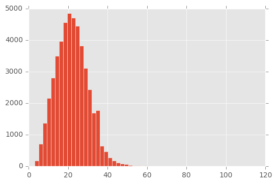
For the use of neural nets (at least with keras, this is no theoretical reason) we need to use equal-lenght input sequences. So we are going to pad our sentences to a length of 50. But first we need dictionaries of words and tags.
max_len = 50
word2idx = {w: i for i, w in enumerate(words)}
tag2idx = {t: i for i, t in enumerate(tags)}
word2idx["Obama"]
25292
tag2idx["B-geo"]
11
Now we map the sentences to a sequence of numbers and then pad the sequence.
from keras.preprocessing.sequence import pad_sequences
X = [[word2idx[w[0]] for w in s] for s in sentences]
Using TensorFlow backend.
X = pad_sequences(maxlen=max_len, sequences=X, padding="post", value=n_words - 1)
X[1]
array([ 8461, 33837, 21771,  6080, 20007, 11069, 10139, 24950, 11069,
       30594,  3989, 17574, 13378, 15727,  3808, 20200,   230, 27681,
       23901, 21530, 12892,  9370, 12368, 16610, 33447, 35178, 35178,
       35178, 35178, 35178, 35178, 35178, 35178, 35178, 35178, 35178,
       35178, 35178, 35178, 35178, 35178, 35178, 35178, 35178, 35178,
       35178, 35178, 35178, 35178, 35178], dtype=int32)
And we need to do the same for our tag sequence.
y = [[tag2idx[w[2]] for w in s] for s in sentences]
y = pad_sequences(maxlen=max_len, sequences=y, padding="post", value=tag2idx["O"])
y[1]
array([ 2,  5,  5,  5,  5,  5,  5,  5,  5,  5,  5,  5,  5,  5,  5, 16,  5,
        5,  5, 14,  5,  5,  5,  5,  5,  5,  5,  5,  5,  5,  5,  5,  5,  5,
        5,  5,  5,  5,  5,  5,  5,  5,  5,  5,  5,  5,  5,  5,  5,  5], dtype=int32)
For training the network we also need to change the labels $y$ to categorial.
from keras.utils import to_categorical
y = [to_categorical(i, num_classes=n_tags) for i in y]
We split in train and test set.
from sklearn.model_selection import train_test_split
X_tr, X_te, y_tr, y_te = train_test_split(X, y, test_size=0.1)
Build and fit the LSTM model
Now we can fit a LSTM network with an embedding layer.
from keras.models import Model, Input
from keras.layers import LSTM, Embedding, Dense, TimeDistributed, Dropout, Bidirectional
input = Input(shape=(max_len,))
model = Embedding(input_dim=n_words, output_dim=50, input_length=max_len)(input)  # 50-dim embedding
model = Dropout(0.1)(model)
model = Bidirectional(LSTM(units=100, return_sequences=True, recurrent_dropout=0.1))(model)  # variational biLSTM
out = TimeDistributed(Dense(n_tags, activation="softmax"))(model)  # softmax output layer
model = Model(input, out)
model.compile(optimizer="rmsprop", loss="categorical_crossentropy", metrics=["accuracy"])
history = model.fit(X_tr, np.array(y_tr), batch_size=32, epochs=5, validation_split=0.1, verbose=1)
Train on 38846 samples, validate on 4317 samples
Epoch 1/5
38846/38846 [==============================] - 247s - loss: 0.1419 - acc: 0.9640 - val_loss: 0.0630 - val_acc: 0.9815
Epoch 2/5
38846/38846 [==============================] - 250s - loss: 0.0552 - acc: 0.9840 - val_loss: 0.0513 - val_acc: 0.9847
Epoch 3/5
38846/38846 [==============================] - 245s - loss: 0.0462 - acc: 0.9865 - val_loss: 0.0480 - val_acc: 0.9857
Epoch 4/5
38846/38846 [==============================] - 245s - loss: 0.0417 - acc: 0.9878 - val_loss: 0.0462 - val_acc: 0.9859
Epoch 5/5
38846/38846 [==============================] - 246s - loss: 0.0388 - acc: 0.9886 - val_loss: 0.0446 - val_acc: 0.9864
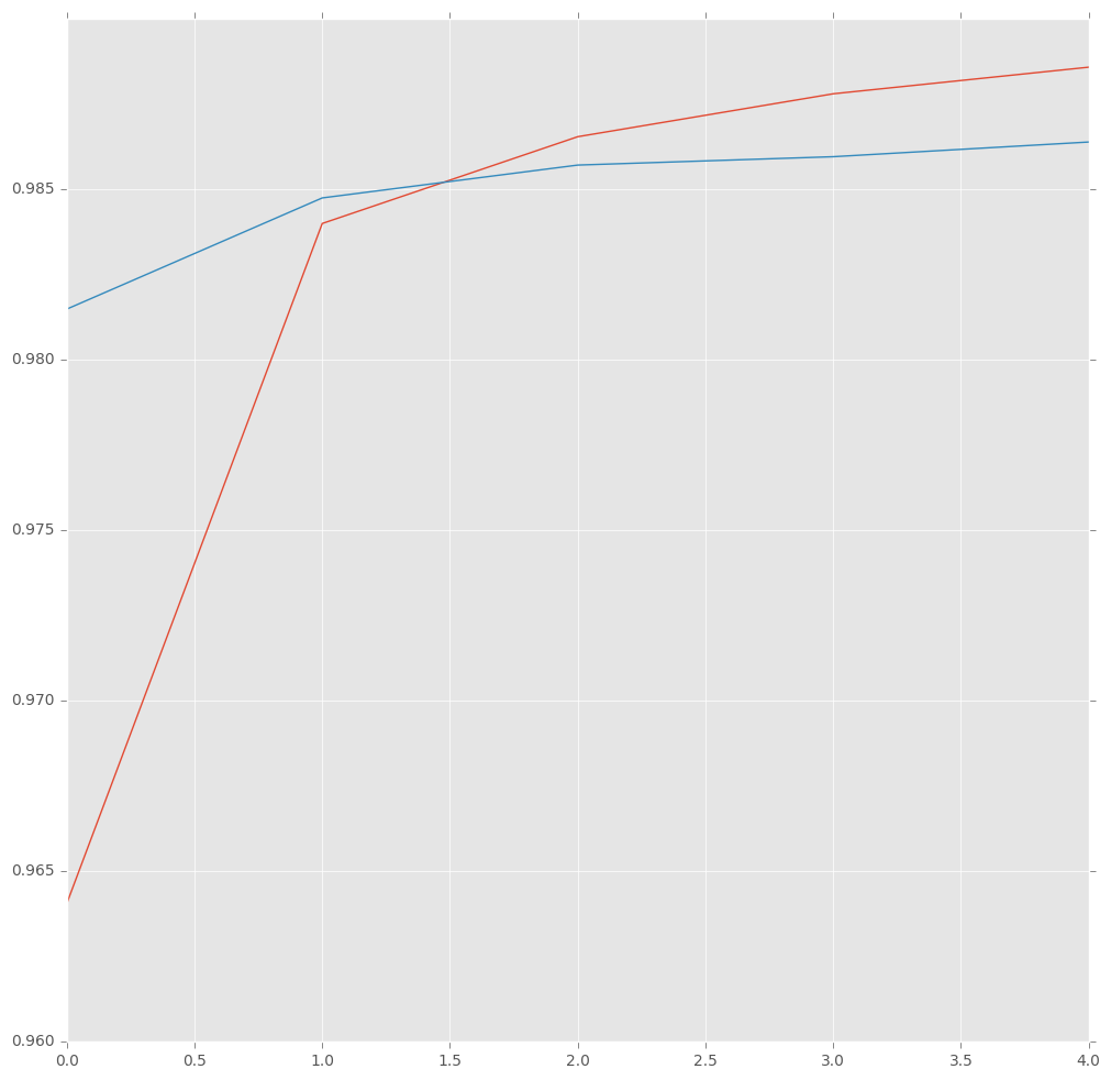
hist = pd.DataFrame(history.history)
plt.figure(figsize=(12,12))
plt.plot(hist["acc"])
plt.plot(hist["val_acc"])
plt.show()
Evaluate the model
Now look at some predictions.
i = 2318
p = model.predict(np.array([X_te[i]]))
p = np.argmax(p, axis=-1)
print("{:15} ({:5}): {}".format("Word", "True", "Pred"))
for w, pred in zip(X_te[i], p[0]):
    print("{:15}: {}".format(words[w], tags[pred]))
Word            (True ): Pred
The            : O
State          : B-org
Department     : I-org
said           : O
Friday         : B-tim
Washington     : B-geo
is             : O
working        : O
with           : O
the            : O
Ethiopian      : B-gpe
government     : O
,              : O
international  : O
partners       : O
and            : O
non-governmental: O
organizations  : O
in             : O
responding     : O
to             : O
concerns       : O
over           : O
humanitarian   : O
conditions     : O
in             : O
the            : O
eastern        : O
region         : O
.              : O
ENDPAD         : O
ENDPAD         : O
ENDPAD         : O
ENDPAD         : O
ENDPAD         : O
ENDPAD         : O
ENDPAD         : O
ENDPAD         : O
ENDPAD         : O
ENDPAD         : O
ENDPAD         : O
ENDPAD         : O
ENDPAD         : O
ENDPAD         : O
ENDPAD         : O
ENDPAD         : O
ENDPAD         : O
ENDPAD         : O
ENDPAD         : O
ENDPAD         : O
This looks pretty good and it did require any feature engineering. So stay tuned for more NLP posts and try some of the proposed methods yourself.