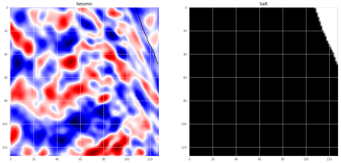
Today I’m going to write about a kaggle competition I started working on recently. In the TGS Salt Identification Challenge, you are asked to segment salt deposits beneath the Earth’s surface. So we are given a set of seismic images that are $101 \times 101$ pixels each and each pixel is classified as either salt or sediment. The goal of the competition is to segment regions that contain salt. A seismic image is produced from imaging the reflection coming from rock boundaries. The seismic image shows the boundaries between different rock types. Lets look at some of the images and the labels now.
import os
import random
import pandas as pd
import numpy as np
import matplotlib.pyplot as plt
plt.style.use("ggplot")
%matplotlib inline

from tqdm import tqdm_notebook, tnrange
from itertools import chain
from skimage.io import imread, imshow, concatenate_images
from skimage.transform import resize
from skimage.morphology import label
from sklearn.model_selection import train_test_split

import tensorflow as tf

from keras.models import Model, load_model
from keras.layers import Input, BatchNormalization, Activation, Dense, Dropout
from keras.layers.core import Lambda, RepeatVector, Reshape
from keras.layers.convolutional import Conv2D, Conv2DTranspose
from keras.layers.pooling import MaxPooling2D, GlobalMaxPool2D
from keras.layers.merge import concatenate, add
from keras.callbacks import EarlyStopping, ModelCheckpoint, ReduceLROnPlateau
from keras.optimizers import Adam
from keras.preprocessing.image import ImageDataGenerator, array_to_img, img_to_array, load_img
# Set some parameters
im_width = 128
im_height = 128
border = 5
path_train = '../input/train/'
path_test = '../input/test/'
Load the images
# Get and resize train images and masks
def get_data(path, train=True):
    ids = next(os.walk(path + "images"))[2]
    X = np.zeros((len(ids), im_height, im_width, 1), dtype=np.float32)
    if train:
        y = np.zeros((len(ids), im_height, im_width, 1), dtype=np.float32)
    print('Getting and resizing images ... ')
    for n, id_ in tqdm_notebook(enumerate(ids), total=len(ids)):
        # Load images
        img = load_img(path + '/images/' + id_, grayscale=True)
        x_img = img_to_array(img)
        x_img = resize(x_img, (128, 128, 1), mode='constant', preserve_range=True)

        # Load masks
        if train:
            mask = img_to_array(load_img(path + '/masks/' + id_, grayscale=True))
            mask = resize(mask, (128, 128, 1), mode='constant', preserve_range=True)

        # Save images
        X[n, ..., 0] = x_img.squeeze() / 255
        if train:
            y[n] = mask / 255
    print('Done!')
    if train:
        return X, y
    else:
        return X

X, y = get_data(path_train, train=True)
# Split train and valid
X_train, X_valid, y_train, y_valid = train_test_split(X, y, test_size=0.15, random_state=2018)
# Check if training data looks all right
ix = random.randint(0, len(X_train))
has_mask = y_train[ix].max() > 0

fig, ax = plt.subplots(1, 2, figsize=(20, 10))

ax[0].imshow(X_train[ix, ..., 0], cmap='seismic', interpolation='bilinear')
if has_mask:
    ax[0].contour(y_train[ix].squeeze(), colors='k', levels=[0.5])
ax[0].set_title('Seismic')

ax[1].imshow(y_train[ix].squeeze(), interpolation='bilinear', cmap='gray')
ax[1].set_title('Salt');
The UNet model
A successful and popular model for these kind of problems is the UNet architecture. The network architecture is illustrated in Figure 1. It consists of a contracting path (left side) and an expansive path (right side).
- The contracting path follows the typical architecture of a convolutional network. It consists of the repeated application of two $3\times3$ convolutions, each followed by a batchnormalization layer and a rectified linear unit (ReLU) activation and dropout and a $2\times2$ max pooling operation with stride $2$ for downsampling. At each downsampling step we double the number of feature channels. The purpose of this contracting path is to capture the context of the input image in order to be able to do segmentation.
- Every step in the expansive path consists of an upsampling of the feature map followed by a $2\times2$ convolution (“up-convolution”) that halves the number of feature channels, a concatenation with the correspondingly feature map from the contracting path, and two $3\times3$ convolutions, each followed by batchnorm, dropout and a ReLU. The purpose of this expanding path is to enable precise localization combined with contextual information from the contracting path.
- At the final layer a $1\times1$ convolution is used to map each $16$-component feature vector to the desired number of classes.

def conv2d_block(input_tensor, n_filters, kernel_size=3, batchnorm=True):
    # first layer
    x = Conv2D(filters=n_filters, kernel_size=(kernel_size, kernel_size), kernel_initializer="he_normal",
               padding="same")(input_tensor)
    if batchnorm:
        x = BatchNormalization()(x)
    x = Activation("relu")(x)
    # second layer
    x = Conv2D(filters=n_filters, kernel_size=(kernel_size, kernel_size), kernel_initializer="he_normal",
               padding="same")(x)
    if batchnorm:
        x = BatchNormalization()(x)
    x = Activation("relu")(x)
    return x
def get_unet(input_img, n_filters=16, dropout=0.5, batchnorm=True):
    # contracting path
    c1 = conv2d_block(input_img, n_filters=n_filters*1, kernel_size=3, batchnorm=batchnorm)
    p1 = MaxPooling2D((2, 2)) (c1)
    p1 = Dropout(dropout*0.5)(p1)

    c2 = conv2d_block(p1, n_filters=n_filters*2, kernel_size=3, batchnorm=batchnorm)
    p2 = MaxPooling2D((2, 2)) (c2)
    p2 = Dropout(dropout)(p2)

    c3 = conv2d_block(p2, n_filters=n_filters*4, kernel_size=3, batchnorm=batchnorm)
    p3 = MaxPooling2D((2, 2)) (c3)
    p3 = Dropout(dropout)(p3)

    c4 = conv2d_block(p3, n_filters=n_filters*8, kernel_size=3, batchnorm=batchnorm)
    p4 = MaxPooling2D(pool_size=(2, 2)) (c4)
    p4 = Dropout(dropout)(p4)

    c5 = conv2d_block(p4, n_filters=n_filters*16, kernel_size=3, batchnorm=batchnorm)

    # expansive path
    u6 = Conv2DTranspose(n_filters*8, (3, 3), strides=(2, 2), padding='same') (c5)
    u6 = concatenate([u6, c4])
    u6 = Dropout(dropout)(u6)
    c6 = conv2d_block(u6, n_filters=n_filters*8, kernel_size=3, batchnorm=batchnorm)

    u7 = Conv2DTranspose(n_filters*4, (3, 3), strides=(2, 2), padding='same') (c6)
    u7 = concatenate([u7, c3])
    u7 = Dropout(dropout)(u7)
    c7 = conv2d_block(u7, n_filters=n_filters*4, kernel_size=3, batchnorm=batchnorm)

    u8 = Conv2DTranspose(n_filters*2, (3, 3), strides=(2, 2), padding='same') (c7)
    u8 = concatenate([u8, c2])
    u8 = Dropout(dropout)(u8)
    c8 = conv2d_block(u8, n_filters=n_filters*2, kernel_size=3, batchnorm=batchnorm)

    u9 = Conv2DTranspose(n_filters*1, (3, 3), strides=(2, 2), padding='same') (c8)
    u9 = concatenate([u9, c1], axis=3)
    u9 = Dropout(dropout)(u9)
    c9 = conv2d_block(u9, n_filters=n_filters*1, kernel_size=3, batchnorm=batchnorm)

    outputs = Conv2D(1, (1, 1), activation='sigmoid') (c9)
    model = Model(inputs=[input_img], outputs=[outputs])
    return model
Since dropout seems not to work well for me in this competition we set it to a low value. Batchnormalization improves the training quite a lot.
input_img = Input((im_height, im_width, 1), name='img')
model = get_unet(input_img, n_filters=16, dropout=0.05, batchnorm=True)

model.compile(optimizer=Adam(), loss="binary_crossentropy", metrics=["accuracy"])
model.summary()
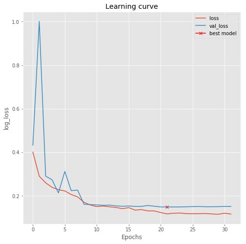
Now we can train the model. We use some callbacks to save the model while training, lower the learning rate if the validation loss plateaus and perform early stopping.
callbacks = [
    EarlyStopping(patience=10, verbose=1),
    ReduceLROnPlateau(factor=0.1, patience=3, min_lr=0.00001, verbose=1),
    ModelCheckpoint('model-tgs-salt.h5', verbose=1, save_best_only=True, save_weights_only=True)
]
results = model.fit(X_train, y_train, batch_size=32, epochs=100, callbacks=callbacks,
                    validation_data=(X_valid, y_valid))
plt.figure(figsize=(8, 8))
plt.title("Learning curve")
plt.plot(results.history["loss"], label="loss")
plt.plot(results.history["val_loss"], label="val_loss")
plt.plot( np.argmin(results.history["val_loss"]), np.min(results.history["val_loss"]), marker="x", color="r", label="best model")
plt.xlabel("Epochs")
plt.ylabel("log_loss")
plt.legend();
Inference with the model
Now we can load the best model we saved and look at some predictions.
# Load best model
model.load_weights('model-tgs-salt.h5')
# Evaluate on validation set (this must be equals to the best log_loss)
model.evaluate(X_valid, y_valid, verbose=1)
# Predict on train, val and test
preds_train = model.predict(X_train, verbose=1)
preds_val = model.predict(X_valid, verbose=1)

# Threshold predictions
preds_train_t = (preds_train > 0.5).astype(np.uint8)
preds_val_t = (preds_val > 0.5).astype(np.uint8)
An important step we skip here is to select an appropriate threshold for the model. This is normally done by optimizing the threshold on a holdout set. Let’s look at some predictions.
def plot_sample(X, y, preds, binary_preds, ix=None):
    if ix is None:
        ix = random.randint(0, len(X))

    has_mask = y[ix].max() > 0

    fig, ax = plt.subplots(1, 4, figsize=(20, 10))
    ax[0].imshow(X[ix, ..., 0], cmap='seismic')
    if has_mask:
        ax[0].contour(y[ix].squeeze(), colors='k', levels=[0.5])
    ax[0].set_title('Seismic')

    ax[1].imshow(y[ix].squeeze())
    ax[1].set_title('Salt')

    ax[2].imshow(preds[ix].squeeze(), vmin=0, vmax=1)
    if has_mask:
        ax[2].contour(y[ix].squeeze(), colors='k', levels=[0.5])
    ax[2].set_title('Salt Predicted')

    ax[3].imshow(binary_preds[ix].squeeze(), vmin=0, vmax=1)
    if has_mask:
        ax[3].contour(y[ix].squeeze(), colors='k', levels=[0.5])
    ax[3].set_title('Salt Predicted binary');
# Check if training data looks all right
plot_sample(X_train, y_train, preds_train, preds_train_t, ix=14)

# Check if valid data looks all right
plot_sample(X_valid, y_valid, preds_val, preds_val_t, ix=19)
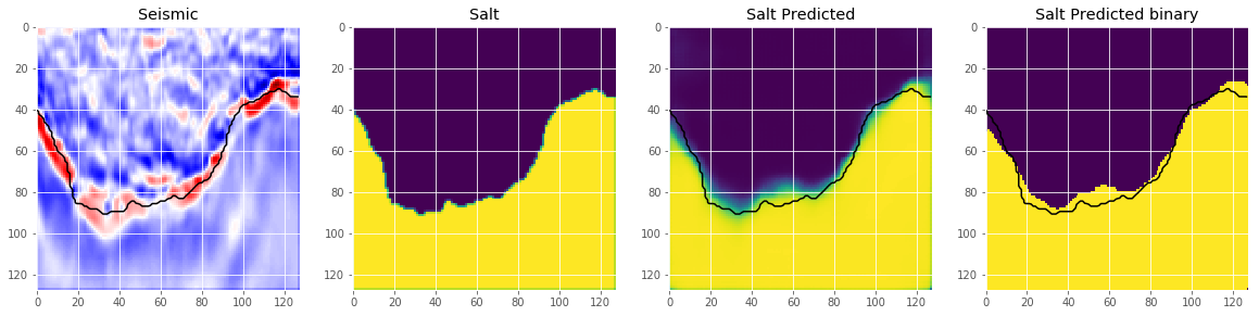
This looks like we are going in the right direction, but obviously there is space left to improve. But that’s it for now. Now you can use the model to predict on the test images and submit your predictions to the competition. If you use an appropriate method to choose the threshold, this should give you a score around $0.7$ on the leaderboard.
I hope you enjoyed this post and learned something. Join the competition and try the model yourself. In the next post, I will show you how to improve the model with data augmentation and cyclical learning rates.